A noisy start
I was sure I had released this… Honestly, I thought the new version of ambient had landed on CRAN a year ago. What does that say about me as a developer? Probably not something very positive. One reason is probably that ambient is one of my smaller packages mostly made for myself. It generates noise patterns which is something I use extensively in my generative art. And the version of ambient I’m now announcing has been available on my own computer for a long time, so I haven’t noticed the lack of a real CRAN release.
What is noise
Anyway, what is this package really about? It is a package that facilitates the generation of multidimensional noise of different kinds. Noise should not be equated with completely random values, R has extensive support for generating these through the different distribution sampling functions. The noise that ambient is capable of producing are random, but spatially correlated noise patterns… what on earth is that? Let’s have a look!
library(ambient)
library(dplyr)

image(noise_perlin(dim = c(300, 400)))
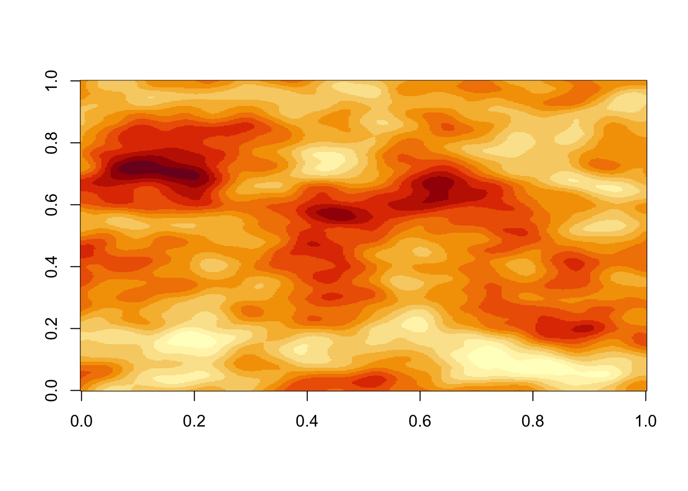
We see in the above example that the pattern is sort of random, but it remains structured so the value at each point is highly correlated to its neighbors. While we have looked at a 2D example, this principle can be expanded to 3 or even 4 dimensions.
The example above used the old interface which is already available on CRAN. That interface simply returns matrices or arrays with the x and y (and z and t) values corresponding to the indices of each cell. This is fast, but super limiting, and the new and promoted interface that you’ll see in a second adds much more control and power.
A new API
The limitation of the old API was mainly that you were bound to only retrieve values at integer coordinates. This in turn limited the amount of weird operations you might want to do to the coordinates before using them to calculate a noise value. Further, it simply felt clunky and didn’t fit in very well with any type of function composition.
The new API (the old still exists) is centered around a long-format grid representation that you create with long_grid(). It basically creates an adorned data frame with coordinates for each row, but provides additional functionality for converting back to matrix/arrays and raster object:
grid <- long_grid(x = seq(0, 1, length.out = 1000),
                  y = seq(0, 1, length.out = 1000))

grid
## # A tibble: 1,000,000 x 2
## x y
## <dbl> <dbl>
## 1 0 0
## 2 0 0.00100
## 3 0 0.00200
## 4 0 0.00300
## 5 0 0.00400
## 6 0 0.00501
## 7 0 0.00601
## 8 0 0.00701
## 9 0 0.00801
## 10 0 0.00901
## # … with 999,990 more rows
You can create higher dimensions by simply providing z and t arguments to long_grid() as well. This is all kind of boring of course since we haven’t added any noise yet (which is kinda the point of all this). Don’t worry - it will come.
The generators
There are many different types of noise that can be generated with ambient. Perlin noise is perhaps the most well-known (it did land the creator an Oscar after all), but many other exists with different characteristics. All of these can be sampled with the new family of gen_*() functions (generator functions). These all take coordinates along with different other arguments such as e.g. frequency and seed. As an example lets calculate some worley noise:
grid <- grid %>%
  mutate(
    noise = gen_worley(x, y, frequency = 5, value = 'distance')
  )
grid
## # A tibble: 1,000,000 x 3
## x y noise
## <dbl> <dbl> <dbl>
## 1 0 0 0.203
## 2 0 0.00100 0.207
## 3 0 0.00200 0.211
## 4 0 0.00300 0.215
## 5 0 0.00400 0.219
## 6 0 0.00501 0.223
## 7 0 0.00601 0.228
## 8 0 0.00701 0.232
## 9 0 0.00801 0.236
## 10 0 0.00901 0.241
## # … with 999,990 more rowsWe have now created a new column with the respective worley noise value for each cell. It is usually easier to understand by looking at it:
grid %>%
  plot(noise)
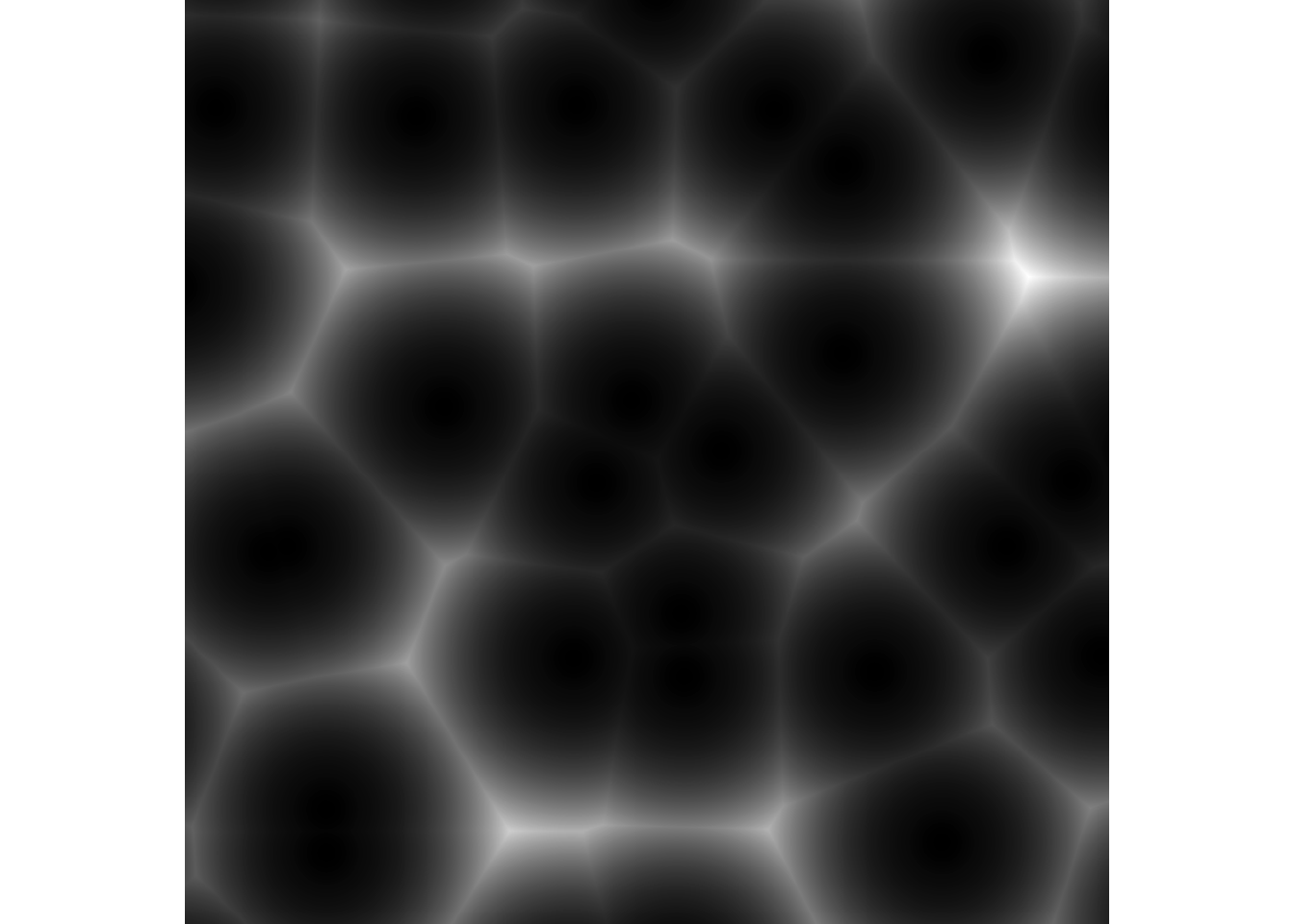
We see that the as.raster() method takes an expression that defines what value should be used for the raster. We normalize it so that it lies between 0 and 1 (a requirement of the raster class) and then use the plot method provided for the raster class.
There are a bunch of these gen_() functions. Further, there are also a bunch of gen_() functions for creating non-noise patterns, e.g.
grid %>%
  mutate(
    pattern = gen_waves(x, y, frequency = 5)
  ) %>%
  plot(pattern)

You may feel at this point that the old interface was much nicer, but the great thing about the generators is that they don’t care about whether the coordinates you feed into it lie in a grid. This means that they can be used to directly look up noise values for particles in a simulation, or modify the grid coordinates before they are passed into the generator. The latter is what is known as noise perturbation and was only available in a very limited form in the old API.
grid %>%
  mutate(
    pertube = gen_simplex(x, y, frequency = 5) / 10,
    noise = gen_worley(x + pertube, y + pertube, value = 'distance', frequency = 5)
  ) %>%
  plot(noise)
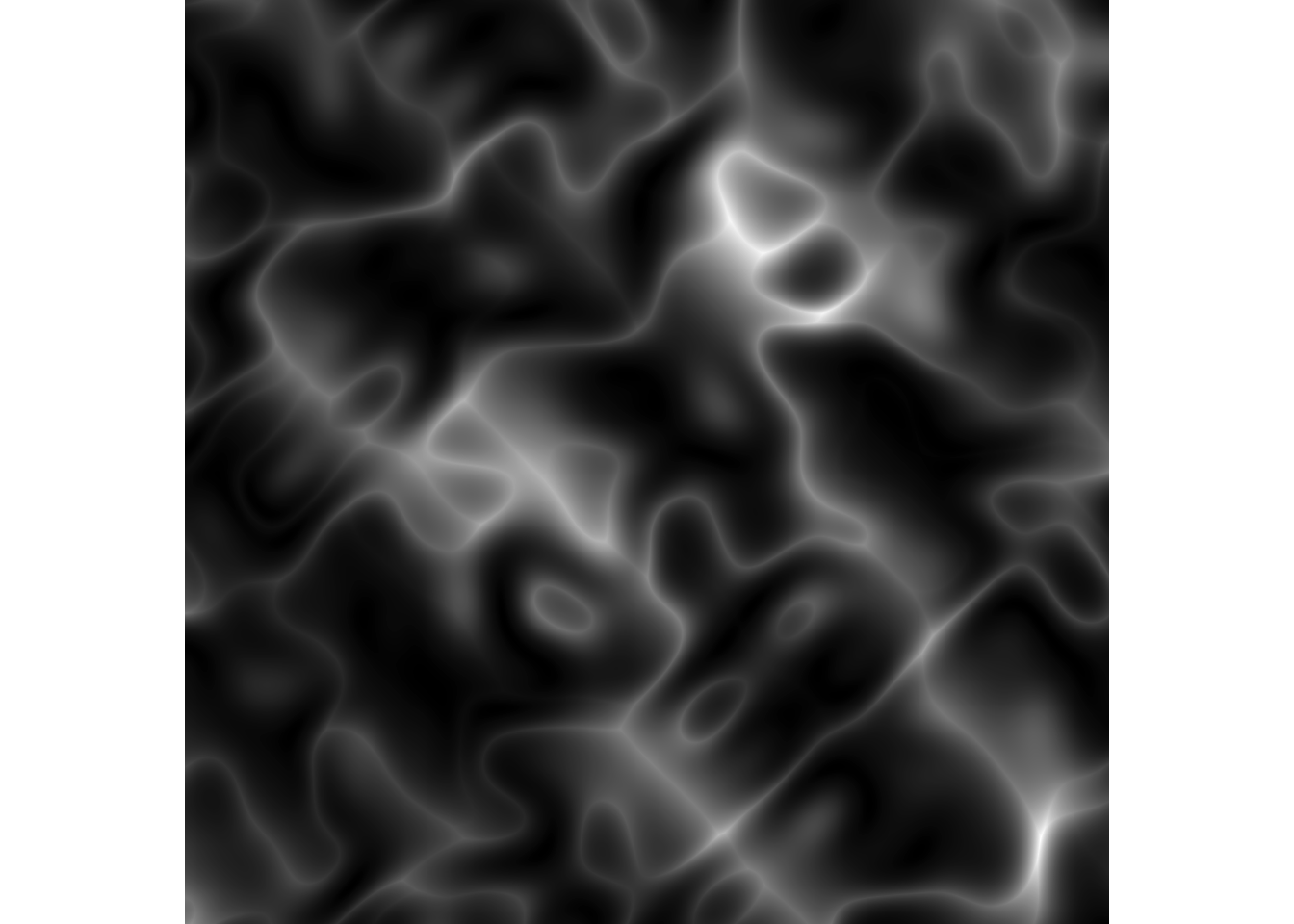
Funky, right? Just to explain what is really going on, each cell in the grid gets a simplex based value, which it then uses to offset its own coordinates before looking up its worley noise value. As simplex noise has a smooth gradient we get these waves distortions of the worley noise.
Fractured noise
The output of e.g. gen_perlin() does not look like what you’d expect if you are used to working with perlin noise (I’d guess). This is because perlin noise is most often used in its fractal form. Fractal noise simply means calculating multiple values for each coordinates at different frequencies and somehow combining them. The most well known is fractal brownian motion (fbm) that simply adds each value together with decreasing intensity, but any combination scheme is possible and ambient comes with a few. To create fractal noise with the new interface we use the fracture() method and pass in a generator and a fractal function along with the different arguments to it:
# Classic perlin noise (combining 4 different frequencies)
grid %>%
  mutate(
    noise = fracture(gen_perlin, fbm, octaves = 4, x = x, y = y, freq_init = 5)
  ) %>%
  plot(noise)
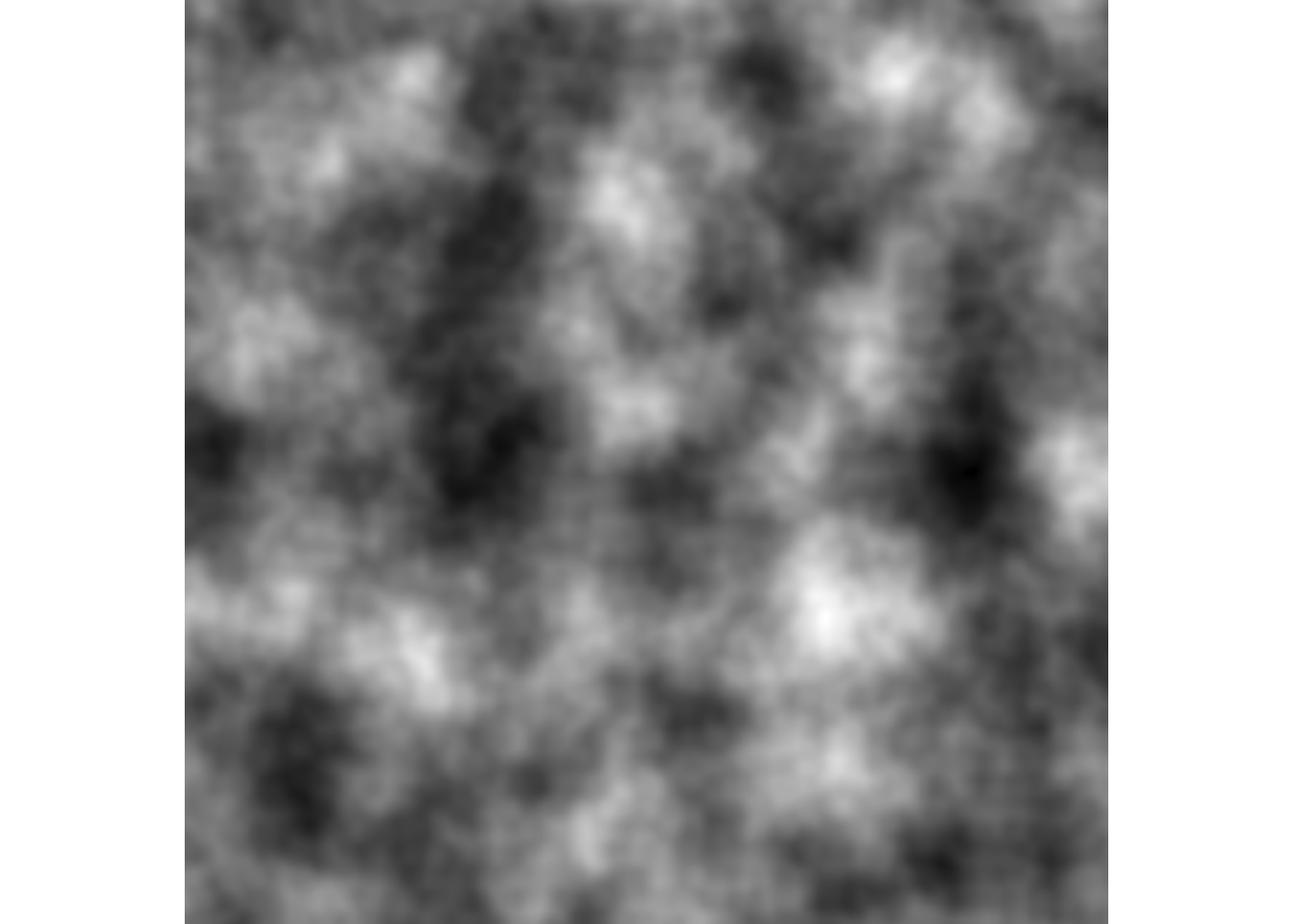
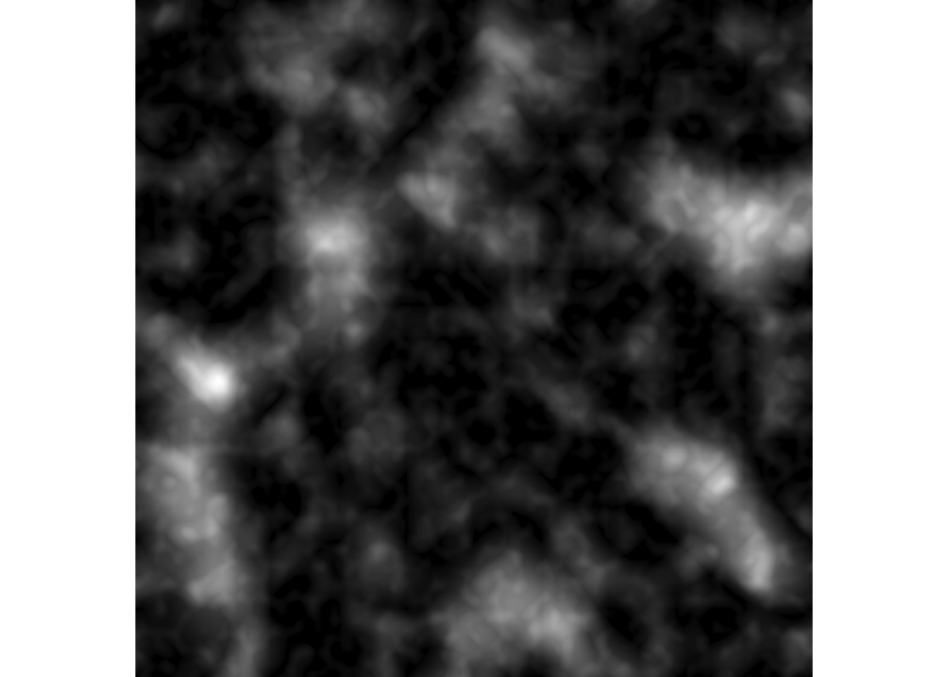
ambient comes with a handful of different fractal function and you can create your own as well
# clamp noise before adding them together
grid %>%
  mutate(
    noise = fracture(gen_perlin, clamped, octaves = 4, x = x, y = y, freq_init = 5)
  ) %>%
  plot(noise)
There are a few other functions as part of this release for e.g. blending values together and calculating derived values from noise fields (e.g. curl and gradient). I will let it be up to you to explore these at your own accord.