Vectorising like a (semi)pro
This is a short practical post about programming with R. Take it for what it is and nothing more…
R is slow! That is what they keep telling us (they being someone who “knows” about “real” programming and has another language that they for some reason fail to be critical about).
R is a weird thing. Especially for people who has been trained in a classical programming language. One of the main reasons for this is its vectorised nature, which is not just about the fact that vectors are prevalent in the language, but is an underlying principle that should guide the design of efficient algorithms in the language. IF you write R like you write C (or Python), then sure it is slow, but really, you are just using it wrong.
This post will take you through the design of a vectorised function. The genesis of the function comes from my generative art, but I thought it was so nice and self-contained that it would make a good blog post. If that seems like something that could take your mind off the pandemic, then buckle up!
The problem
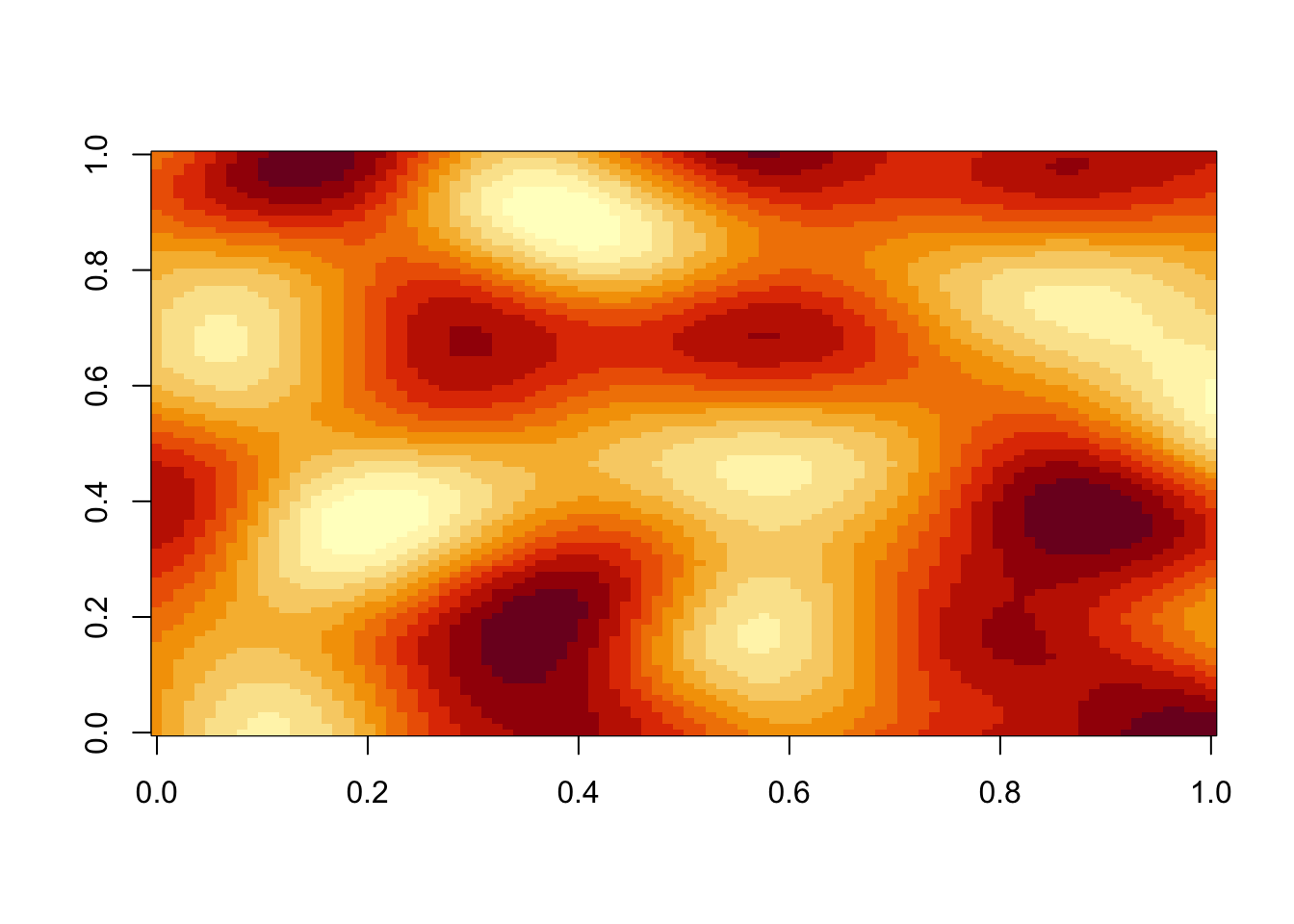
I have a height-map, that is, a matrix of numeric values. You know what? Let’s make this concrete and create one:
library(ambient)
library(dplyr)

z <- long_grid(1:100, 1:100) %>%
  mutate(val = gen_simplex(x, y, frequency = 0.02)) %>%
  as.matrix(val)

image(z, useRaster = TRUE)

This is just some simplex noise of course, but it fits our purpose…
Anyway, we have a height-map and we want to find the local extrema, that is, the local minimum and maximum. That’s it. Quite a simple and understandable challenge right.
Vectorised, smecktorised
Now, had you been a trained C-programmer you would probably have solved this with a loop. This is the way it should be done in C, but applying this to R will result in a very annoyed programmer who will tell anyone who cares to listen that R is slow.
We already knew this. We want something vectorised, right? But what is vectorised anyway? All over the internet the recommendation is to use the apply()-family of function to vectorise your code, but I have some bad news for you: This is the absolute wrong way to vectorise. There are a lot of good reasons to use the functional approach to looping instead of the for-loop, but when it comes to R, performance is not one of them.
Shit…
To figure this out, we need to be a bit more clear about what we mean with a vectorised function. There are some different ways to think about it
-
The broad and lazy definition is a function that operates on the elements of a vector. This is where
apply()(and friends) based functions reside. - The narrow and performant definition is a function that operates on the elements of a vector in compiled code. This is where many of R’s base functions live along with properly designed functions implemented in C or C++
- The middle ground is a function that is composed of calls to 2. to avoid explicit loops, thus deferring most element-wise operations to compiled code.
We want to talk about 3.. Simply implementing this in compiled code would be cheating, and we wouldn’t learn anything.
Thinking with vectors
R comes with a lot of batteries included. Some of the more high-level function are not implemented with performance in mind (sadly), but a lot of the basic stuff is, e.g. indexing, arithmetic, summations, etc. It turns out that these are often enough to implement pretty complex functions in an efficient vectorised manner.
Going back to our initial problem of finding extrema: What we effectively are asking for is a moving window function where each cell is evaluated on whether it is the largest or smallest value in its respective window. If you think a bit about this, this is mainly an issue of indexing. For each element in the matrix, we want the indices of all the cells within its window. Once we have that, it is pretty easy to extract all the relevant values and use the vectorised pmin() and pmax() function to figure out the maximum value in the window and use the (vectorised) == to see if the extrema is equivalent to the value of the cell.
That’s a lot of talk, here is the final function:
extrema <- function(z, neighbors = 2) {
  ind <- seq_along(z)
  rows <- row(z)
  cols <- col(z)
  n_rows <- nrow(z)
  n_cols <- ncol(z)
  window_offsets <- seq(-neighbors, neighbors)
  window <- outer(window_offsets, window_offsets * n_rows, `+`)
  window_row <- rep(window_offsets, length(window_offsets))
  window_col <- rep(window_offsets, each = length(window_offsets))
  windows <- mapply(function(i, row, col) {
    row <- rows + row
    col <- cols + col
    new_ind <- ind + i
    new_ind[row < 1 | row > n_rows | col < 1 | col > n_cols] <- NA
    z[new_ind]
  }, i = window, row = window_row, col = window_col, SIMPLIFY = FALSE)
  windows <- c(windows, list(na.rm = TRUE))
  minima <- do.call(pmin, windows) == z
  maxima <- do.call(pmax, windows) == z
  extremes <- matrix(0, ncol = n_cols, nrow = n_rows)
  extremes[minima] <- -1
  extremes[maxima] <- 1
  extremes
}
(don’t worry, we’ll go through it in a bit)
This function takes a matrix, and a neighborhood radius and returns a new matrix of the same dimensions as the input, with 1 in the local maxima, -1 in the local minima, and 0 everywhere else.
Let’s go through it:
# ...
  ind <- seq_along(z)
  rows <- row(z)
  cols <- col(z)
  n_rows <- nrow(z)
  n_cols <- ncol(z)
# ...
Here we are simply doing some quick calculations upfront for reuse later. The ind variable is simply the index for each cell in the matrix. Matrices are simply vectors underneath, so they can be indexed like that as well. rows and cols holds the row and column index of each cell, and n_rows and n_cols are pretty self-explanatory.
# ...
  window_offsets <- seq(-neighbors, neighbors)
  window <- outer(window_offsets, window_offsets * n_rows, `+`)
  window_row <- rep(window_offsets, length(window_offsets))
  window_col <- rep(window_offsets, each = length(window_offsets))
# ...
Most of the magic happens here, but it is not that apparent. What we do is that we use the outer() function to construct a matrix, the size of our window, holding the index offset from the center for each of the cells in the window. We also construct vectors holding the rows and column offset for each cell
# ...
  windows <- mapply(function(i, row, col) {
    row <- rows + row
    col <- cols + col
    new_ind <- ind + i
    new_ind[row < 1 | row > n_rows | col < 1 | col > n_cols] <- NA
    z[new_ind]
  }, i = window, row = window_row, col = window_col, SIMPLIFY = FALSE)
# ...
This is where all the magic appear to happen. For each cell in the window, we are calculating it’s respective value for each cell in the input matrix. I can already hear you scream about me using and apply()-like function, but the key thing is that I’m not using it to loop over the elements of the input vector (or matrix), but over a much smaller (and often fixed) number of elements.
If you want to leave now because I’m moving the goal-posts by my guest.
Anyway, what is happening inside the mapply() call? Inside the function we figure out which row and column the offsetted cell is part of. Then we calculate the index of the cells for the offset. In order to guard against out-of-bounds errors we set all the indices that are out of bound to NA, and then we simply index into our matrix. The crucial part is that all of the operations here are vectorised (indexing, arithmetic, and comparisons). In the end we get a list holding vectors of values for each cell in the window.
# ..
  windows <- c(windows, list(na.rm = TRUE))
  minima <- do.call(pmin, windows) == z
  maxima <- do.call(pmax, windows) == z
  extremes <- matrix(0, ncol = n_cols, nrow = n_rows)
  extremes[minima] <- -1
  extremes[maxima] <- 1
  extremes
# ..
This is really just wrapping up, even though the actual computations are happening here. We use pmin() and pmax() to find the maximum and minimum across each window, and compare it to the value in our input matrix (again, all proper vectorised function). In the end we construct a matrix holding 0s and use the calculated positions to set 1 or -1 at the location of local extremes.
Does it work?
I guess that is the million dollar question, closely followed by “is it faster?”. I don’t really care enough to implement a “dumb” vectorisation, so I’ll just put my head on the block with the last question and insist that, yes, it is much faster. You can try to beat me with an apply() based solution and I’ll eat a sticker if you succeed (unless you cheat).
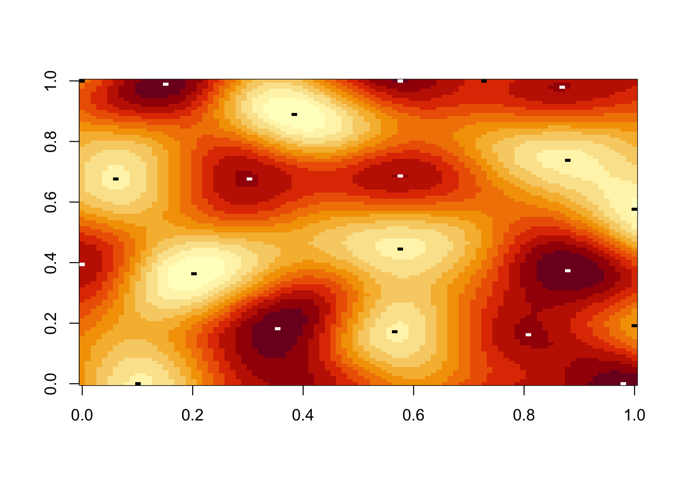
As for the first question, let’s have a look
extremes <- extrema(z)
extremes[extremes == 0] <- NA

image(z, useRaster = TRUE)
image(extremes, col = c('black', 'white'), add = TRUE)

Lo and behold, it appears as if we succeeded.
Can vectorisation save the world?
No…
More to the point, not every problem has a nice vectorised solution. Further, the big downside with proper vectorisation is that it often requires expanding a lot of variables to the size of the input vector. In our case we needed to hold all windows in memory simultaneously, and it does not take too much imagination to think up scenarios where that may make our computer explode. Still, more often than not it is possible to write super performant R code, and usually the crucial part is to figure out how to do some intelligent indexing.
If you are still not convinced then read through Brodie Gaslam’s blog. He has a penchant for implementing ridiculously complicated stuff in highly efficient R code. It goes without saying that his posts are often more involved than this, but if you have kept reading until this point, I think you are ready…