The Colour of Everything

I’m happy to announce that farver 2.0 has landed on CRAN. This is a big release comprising of a rewrite of much of the internals along with a range of new functions and improvements. Read on to find out what this is all about.
The case for farver
The first version of farver really came out of necessity as I identified a major performance bottleneck in gganimate related to converting colours into Lab colour space and back when tweening them. This was a result of grDevices::convertColor() not being meant for use with millions of colour values. I build farver in order to address this very specific need, which in turn made Brodie Gaslam look into speeding up the grDevices function. The bottom line is that, while farver is still the fastest at converting between colour spaces, grDevices is now so fast that I probably wouldn’t have bothered to build farver in the first place had it been like this all along. I find this a prime example of fruitful open source competition and couldn’t be happier that Brodie took it upon him.
So why a new shiny version? As part of removing compiled code from scales, we decided to adopt farver for colour interpolation, and the code could use a brush-up. I’ve become much more trained in writing compiled code, and further there were some shortcomings in the original implementation that needed to be addressed if scales (and thus ggplot2) should depend on it. Further, I usually write on larger frameworks and there is a certain joy in picking a niche area that you care about and go ridiculously overboard in tooling without worrying about if it benefits any other than yourself (ambient is another example of such indulgence).
The new old
The former version of farver was quite limited in functionality. It had two functions: convert_colour() and compare_colour() that did colour space conversion and colour distance calculations respectively. No outward changes has been made to these functions, but internally a lot has happened. The old versions had no input validation, so passing in colours with NA, NaN, Inf, and -Inf would give you some truly weird results back. Further, the input and output was not capped to the range of the given colour space, so you could in theory end up with negative RGB values if you converted from a colour space with a larger gamut than sRGB. Both of these issues has been rectified in the new version. Any non-finite value in any channel will result in NA in all channels in the output (for conversion) or an NA distance (for comparison).
library(farver)
colours <- cbind(r = c(0, NA, 255), g = c(55, 165, 20), b = c(-Inf, 120, 200))
colours
## r g b
## [1,] 0 55 -Inf
## [2,] NA 165 120
## [3,] 255 20 200convert_colour(colours, from = 'rgb', to = 'yxy')## y1 x y2
## [1,] NA NA NA
## [2,] NA NA NA
## [3,] 25.93626 0.385264 0.1924651
Further, input is now capped to the channel range (if any) before conversion, and output is capped again before returning the result. The later means that convert_colour() is only symmetric (ignoring rounding errors) if the colours are within gamut in both colour spaces.
# Equal output because values are capped between 0 and 255
colours <- cbind(r = c(1000, 255), g = 55, b = 120)
convert_colour(colours, 'rgb', 'lab')
## l a b
## [1,] 57.41976 76.10097 12.44826
## [2,] 57.41976 76.10097 12.44826
Lastly, a new colour space has been added: CIELch(uv) (in farver hcl) has been added as a cousin of CIELch(ab) (lch). Both are polar transformations, but the former is based on luv values and the latter on lab. Both colour spaces are used interchangeably (though not equivalent), and as the grDevices::hcl() function is based on the luv space it made sense to provide an equivalent in farver.
The new new
The new functionality mainly revolves around the encoding of colour in text strings. In many programming languages colour can be encoded into strings as #RRGGBB where each channel is given in hexadecimal digits. This is also how colours are passed around in R mostly (R also has a list of recognized colour names that can be given as aliases instead of the hex string - see grDevices::colour() for a list). The encoding is convenient as it allows colours to be encoded into vectors, and thus into data frame columns or arrays, but means that if you need to perform operations on it you’d have to first decode the string into channels, potentially convert it into the required colour space, do the manipulation, convert back to sRGB, and encode it into strings. Encoding and decoding has been supported in grDevices with rgb() and col2rgb() respectively, both of which are pretty fast. col2rgb() has a quirk in that the output has the channels in the rows instead of the columns, contrary to how decoded colours are presented everywhere else:
grDevices::col2rgb(c('#56fec2', 'red'))## [,1] [,2]
## red 86 255
## green 254 0
## blue 194 0farver sports two new functions that, besides providing consistency in the output format also eliminates some steps in the workflow described above:
# Decode strings with decode_colour
colours <- decode_colour(c('#56fec2', 'red'))
colours
## r g b
## [1,] 86 254 194
## [2,] 255 0 0# Encode with encode_colour
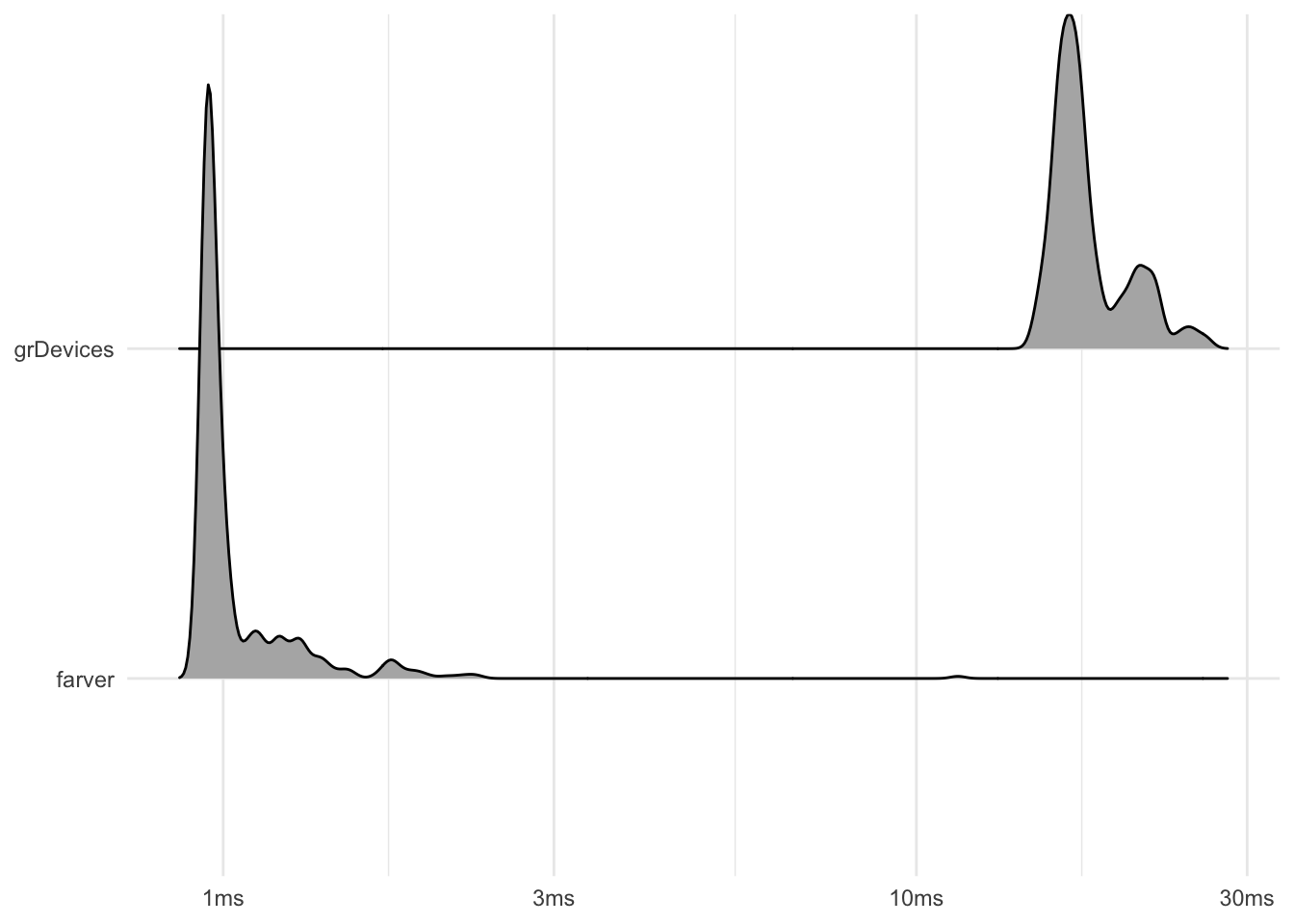
encode_colour(colours)## [1] "#56FEC2" "#FF0000"Besides the basic use shown above, both function allows input/output from other colour spaces than sRGB. That means that if you need to manipulate some colour in Lab space, you can simply decode directly into that, do the manipulation and encode directly back. The functionality is baked into the compiled code, meaning that a lot of memory allocation is spared, making this substantially faster than a grDevices-based workflow:
library(ggplot2)

# Create some random colour strings
colour_strings <- sample(grDevices::colours(), 5000, replace = TRUE)

# Get Lab values from a string
timing <- bench::mark(
  farver = decode_colour(colour_strings, to = 'lab'),
  grDevices = convertColor(t(col2rgb(colour_strings)), 'sRGB', 'Lab', scale.in = 255),
  check = FALSE,
  min_iterations = 100
)
plot(timing, type = 'ridge') +
  theme_minimal() +
  labs(x = NULL, y = NULL)

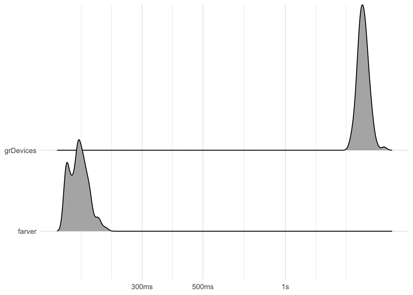
Can we do better than this? If the purpose is simply to manipulate a single channel in a colour encoded as a string, we may forego the encoding and decoding completely and do it all in compiled code. farver provides a family of functions for doing channel manipulation in string encoded colours. The channels can be any channel in any colour space supported by farver, and the decoding, manipulation and encoding is done in one pass. If you have a lot of colours and need to increase e.g. darkness, this can save a lot of memory allocation:
# a lot of colours
colour_strings <- sample(grDevices::colours(), 500000, replace = TRUE)

darken <- function(colour, by) {
  colour <- t(col2rgb(colour))
  colour <- convertColor(colour, from = 'sRGB', 'Lab', scale.in = 255)
  colour[, 'L'] <- colour[, 'L'] * by
  colour <- convertColor(colour, from = 'Lab', to = 'sRGB')
  rgb(colour)
}
timing <- bench::mark(
  farver = multiply_channel(colour_strings, channel = 'l', value = 1.2, space = 'lab'),
  grDevices = darken(colour_strings, 1.2),
  check = FALSE,
  min_iterations = 100
)
plot(timing, type = 'ridge') +
  theme_minimal() +
  labs(x = NULL, y = NULL)

The bottom line
The new release of farver provides invisible improvements to the existing functions and a range of new functionality for working efficiently with string encoded colours. You will be using it indirectly following the next release of scales if you are plotting with ggplot2, but you shouldn’t be able to tell. If you somehow ends up having to manipulate millions of colours, then farver is still the king of the hill by a large margin when it comes to performance, but I personally believe that it also provides a much cleaner API than any of the alternatives.