1 giraffe, 2 giraffe, GO!

I am beyond excited to finally be able to announce a new version of ggraph. This release, like the ggforce 0.3.0 release, has been many years in the making, laying dormant for long periods first waiting for ggplot2 to get updated and then waiting for me to have time to finally finish it off. All that is in the past now as ggraph 2.0.0 has finally landed on CRAN, filled with numerous new features, a massive amount of bug fixes, and a slew of breaking changes.

If you are new to ggraph, a short description follows: It is an extension of ggplot2 that implement an extended grammar for relational data (e.g. trees and networks). It provides a huge variety of geoms for drawing nodes and edges, along with an assortment of layouts making it possible to produce a very wide range of network visualization types. It is to my knowledge the most feature packed network visualization framework available in R (and potentially in other languages as well), all building on top of the familiar ggplot2 API. If you want to learn more I invite you to browse the new pkgdown website that has been made available.

New looks

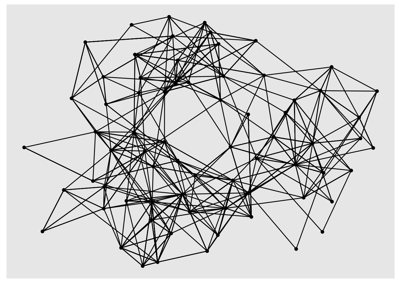
Before we begin with the exiting new stuff, there’s a small change that may or may not greet you as you make your first new plot with ggraph v2.0.0. The default look of a ggplot is often not a good fit for network visualisations as the positional scales are irrelevant. Because of this ggraph has since its release offered a theme_graph() that removed a lot of the useless clutter such as axes and grid lines. You had to use it deliberately though as I didn’t want to overwrite any defaults you may have had. In the new release I’ve relaxed on this a bit. When you construct a ggraph plot it will still use the default theme as a base, but it will remove axes and gridlines from it. This makes it easier to use it together with coorporate templates and the likes right out the box. You can still use theme_graph(), or potentially set it as a default using set_graph_style() if you so wish.

library(ggraph)

# THe new default look:
ggraph(highschool) + 
  geom_edge_link() + 
  geom_node_point()

# Using theme_graph for the remainder of this post
set_graph_style(size = 11, plot_margin = margin(0, 0, 0, 0))

The broken giraffe

Let us start proper with what this release breaks, because it does it for some very good reasons and you’ll all be happy about it shortly as you read on. The 1.x.x versions of ggraph worked with two different types of network representations: igraph objects and dendrogram object. Some further types such as hclust and network objects were supported by automatic conversion, but that was it. Further, the internal architecture meant that certain layouts and geoms could only be used with certain objects. This was obviously an imperfect situation and one that reflected that tidygraph was developed after ggraph. In ggraph 2.0.0 the internals have been rewritten to only be based on tidygraph. This means that all layouts and geoms will always be available (as long as the topology supports it). This doesn’t mean that igraph, dendrogram, network, and hclust objects are no longer supported, though. Every input will be attempted to be coerced to a tbl_graph object, and as tidygraph supports a wealth of network representations, ggraph can now be used with an even wider selection of objects, all completely without any need for change from the user.

While this change was completely internal and thus didn’t break anything, it did put in to question the API of the ggraph() function, which had been designed before tidy evaluation and tidygraph came into existence. Prior to 2.0.0 all layout arguments passed into ggraph() (and create_layout()) would be passed as strings if they referenced any node or edge property, e.g.

library(tidygraph)

graph <- as_tbl_graph(
  data.frame(
    from = sample(5, 20, TRUE),
    to = sample(5, 20, TRUE),
    weight = runif(20)
  )
)

ggraph(graph, layout = 'fr', weights = "weight") + 
  geom_edge_link() + 
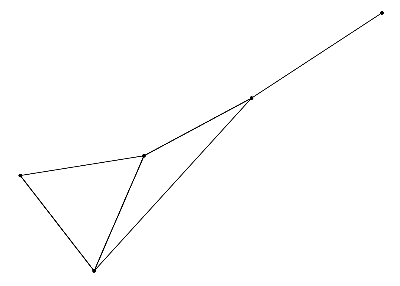
  geom_node_point()

With the new API, edge and node parameters are passed along as unquoted expressions that will be evaluated in the context of the edge or node data respectively. The example above will this be:

ggraph(graph, layout = 'fr', weights = weight) + 
  geom_edge_link() + 
  geom_node_point()

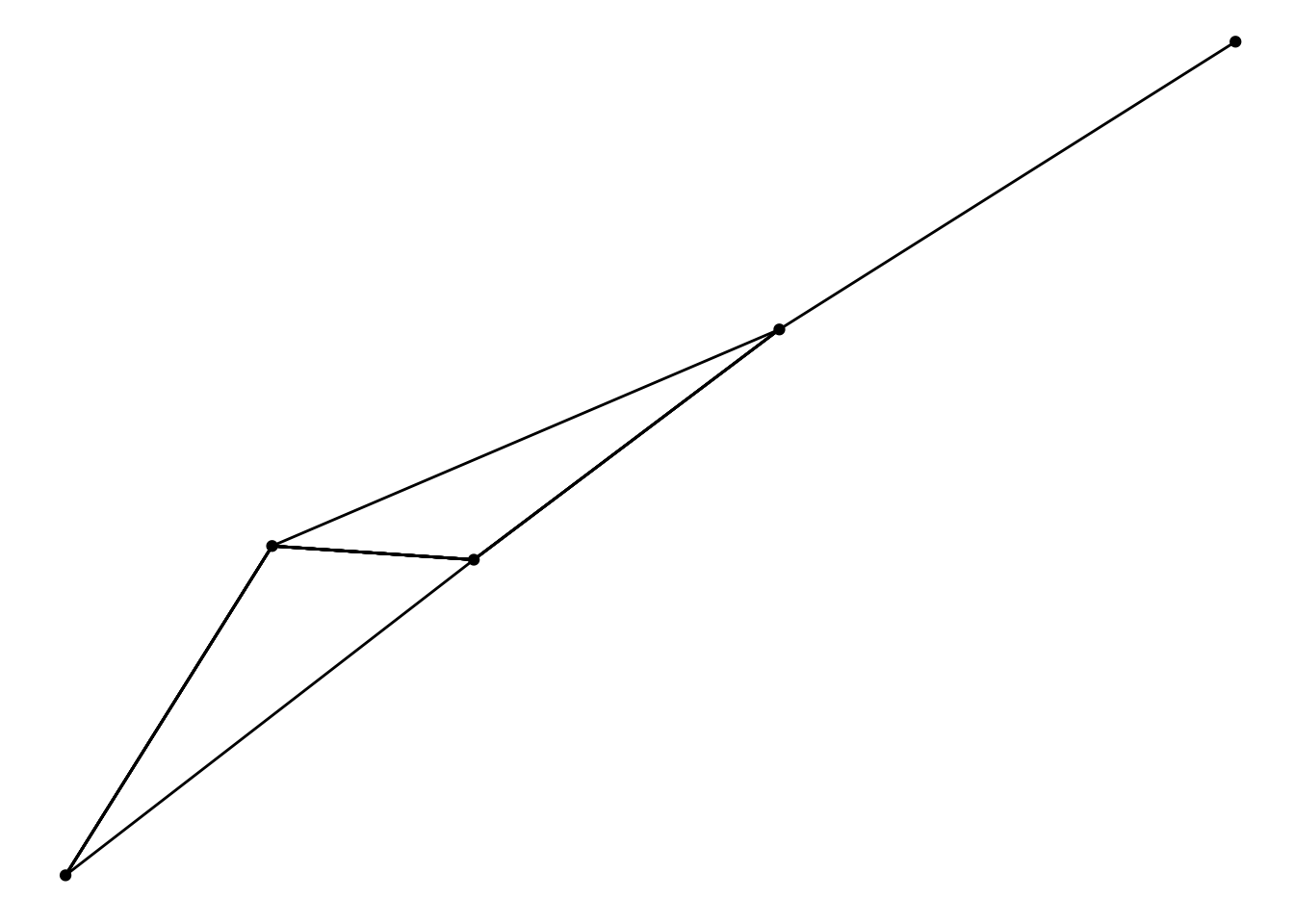
This change might seem superficial and unnecessary until you realize that this means the network object doesn’t have to be updated every time you want to try new edge and node parameters for the layout:

ggraph(graph, layout = 'fr', weights = sqrt(weight)) + 
  geom_edge_link() + 
  geom_node_point()

So, that’s the extent of the breakage… Now what does this change allow..?

Tidygraph inside

The use of tidygraph runs much deeper than simply being used as the internal network representation. ggraph will also register the network object during creation and rendering of the plot, meaning that all tidygraph algorithms are available as input to layout specs and aesthetic mappings:

graph <- as_tbl_graph(highschool)

ggraph(graph, layout = 'fr', weights = centrality_edge_betweenness()) + 
  geom_edge_link() + 
  geom_node_point(aes(size = centrality_pagerank(), colour = node_is_center()))

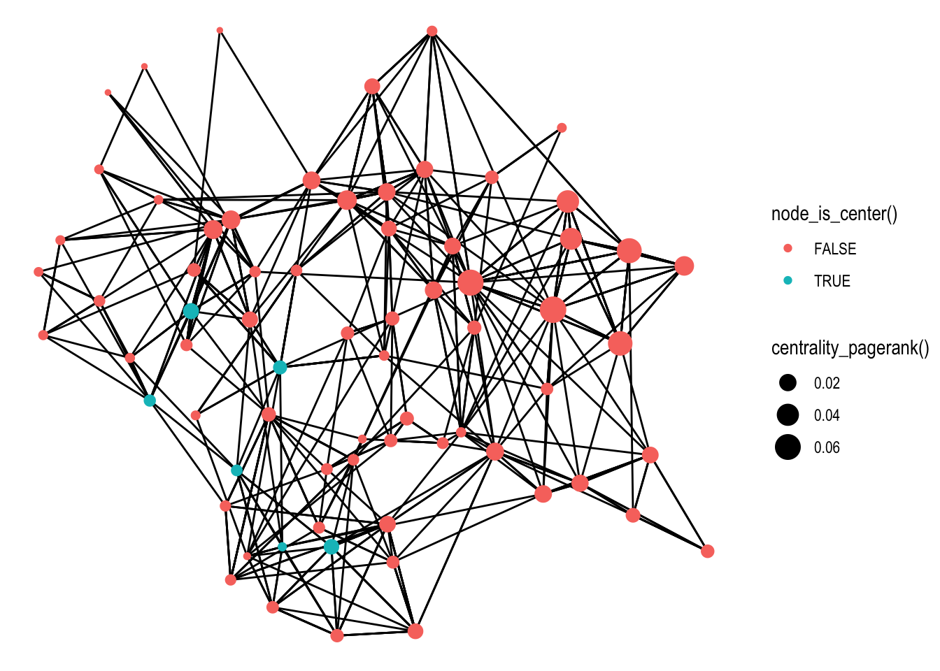
It is obvious (at least to me) that this new-found capability will make it much easier to experiment and iterate on the visualization, hopefully inspiring users to try out different settings before settling on a plot.

As discussed above, the tidygraph integration also makes it easy to plot a wide variety of data types directly. Above we first create a tbl_graph from the highschool edge-list, but that is strictly not necessary:

head(highschool)

##   from to year
## 1    1 14 1957
## 2    1 15 1957
## 3    1 21 1957
## 4    1 54 1957
## 5    1 55 1957
## 6    2 21 1957

ggraph(highschool, layout = 'kk') + 
  geom_edge_link() + 
  geom_node_point()

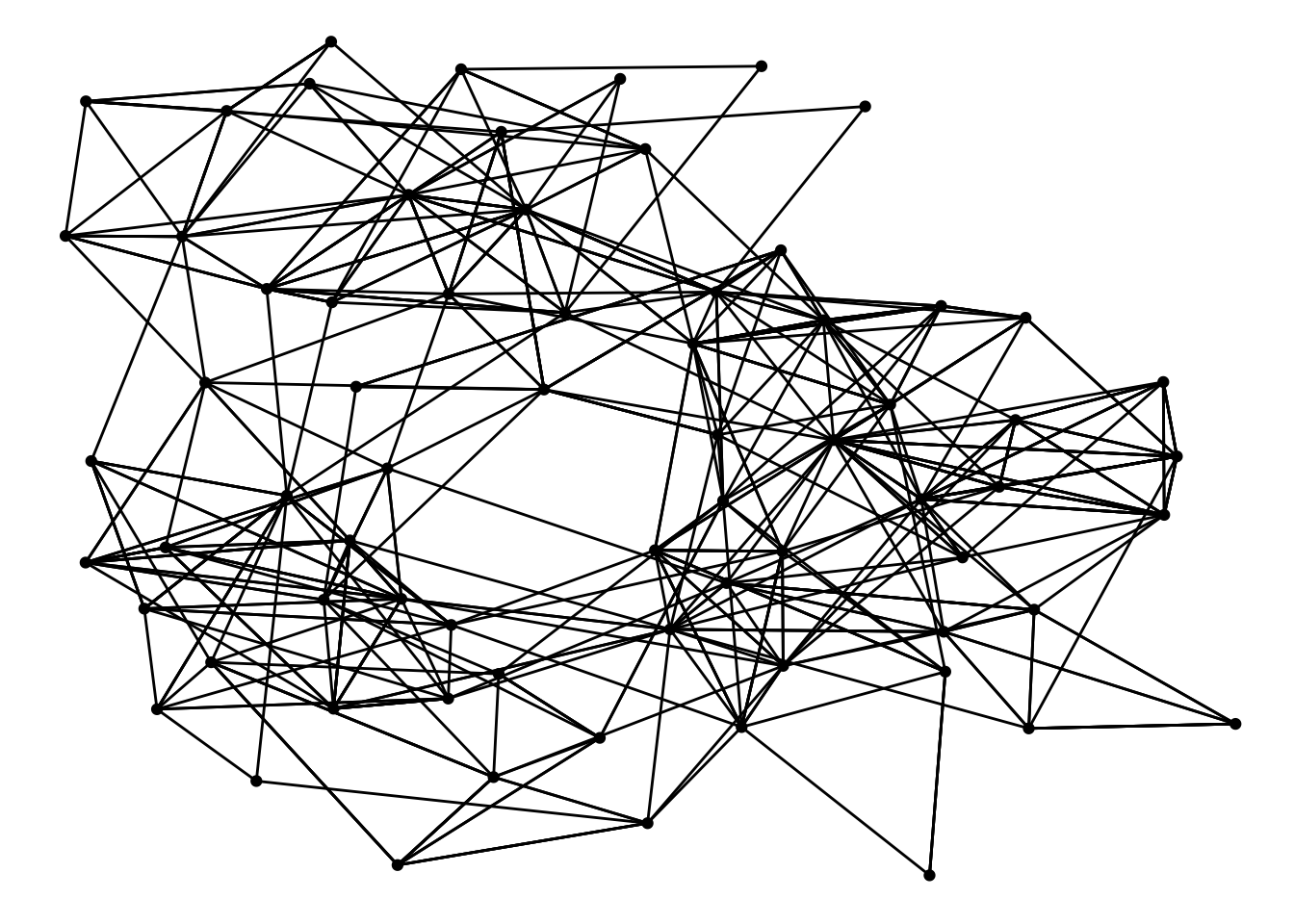
Note that even though the input is not a tbl_graph it will be converted to one so all the tidygraph algorithms are still available during plotting.

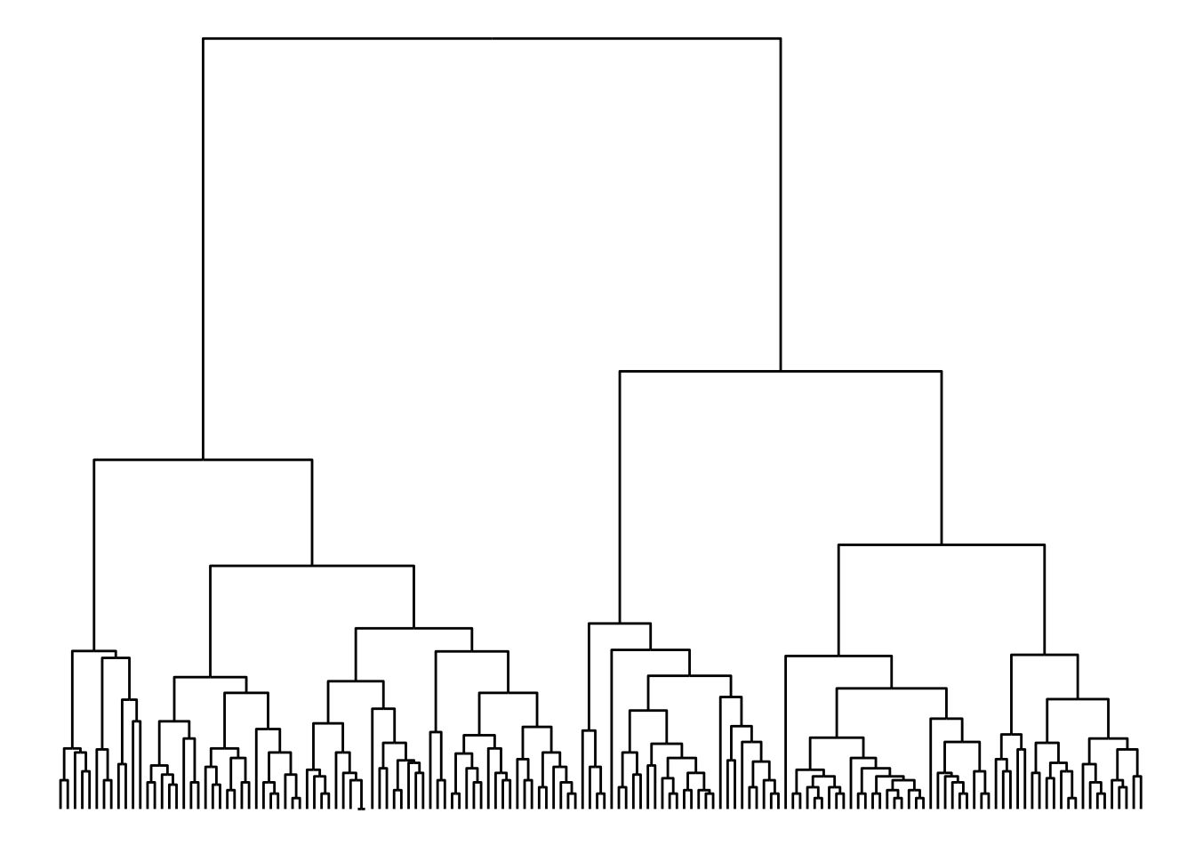
To further make it easy to quickly gain an overview over your network data, ggraph gains a qgraph() function that inspects you input and automatically picks a layout and combination of edge and node geoms. While the return type is a standard ggraph/ggplot object it should not really be used as the basis for a more complicated plot as you have no influence over how the layout and first couple of layers are chosen.

iris_clust <- hclust(dist(iris[, 1:4]))

qgraph(iris_clust)

Layout galore

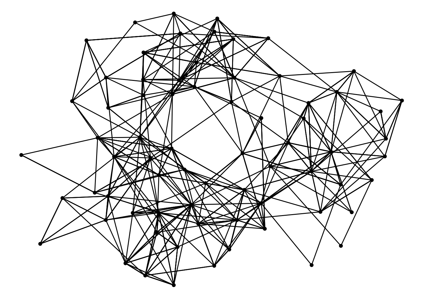
ggraph 2.0.0 comes with a huge selection of new layouts, from new algorithms for the classic node-edge diagram to completely new types such as matrix and (bio)fabric layouts. The biggest addition comes from the integration of the graphlayouts package by David Schoch who has done a tremendous job in bringing new, high quality, layout algorithms to R. The ‘stress’ layout is the new default as it does a much better job than fruchterman-reingold (‘fr’). It also includes a sparse version ‘sparse_stress’ for large graphs that are much faster than any of the ones provided by igraph.

# Defaults to stress, with a message
ggraph(graph) + 
  geom_edge_link() + 
  geom_node_point()

## Using `stress` as default layout

There are other layouts from graphlayouts of interest, e.g. the ‘backbone’ layout that emphasize community structure, the ‘focus’ layout that places all nodes in concentric circle based on their distance to a selected node etc. I wont show them all here but instead direct you to its github page that describes all its different layouts.

Another type of layout that has become available is the unrooted equal-angle and equal-daylight algorithms for drawing unrooted trees. This type of trees are different than those resulting from e.g. hierarchical clustering in that they do not contain direction or a specific root node. The tree structure is only given by the branch length. To support this the ‘dendrogram’ layout has gained a length argument that allows the layout to be calculated from branch length:

library(ape)
data(bird.families)
# Using the bird.orders dataset from ape
ggraph(bird.families, 'dendrogram', length = length) + 
  geom_edge_elbow()

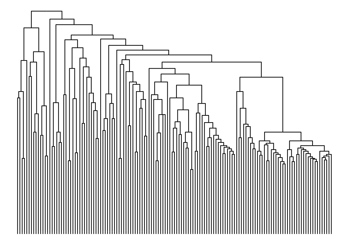
Often the dendrogram layout is a bad choice for unrooted trees, as it implicitly shows a node as the root and draw everything else according to that. Instead one can choose the ‘unrooted’ layout where leafs are attempted evenly spread across the plane.

ggraph(bird.families, 'unrooted', length = length) + 
  geom_edge_link()

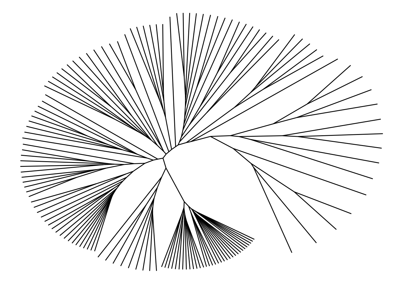
By default the equal-daylight algorithm is used but it is possible to also get the simpler, but less well-dispersed equal-angle version as well by setting daylight = FALSE.

The new version also brings two new special layouts (special meaning non-standard): ‘matrix’ and ‘fabric’, which, like the ‘hive’ layout, brings their own edge and node geoms. The matrix layout places nodes on a diagonal and shows edges by placing points at the horizontal and vertical intersection of the terminal nodes. The selling point of this layout is that it scales better as there is no possibility of edge crossings. On the other hand is matrix layouts very dependent on the order in which nodes are placed, and as the network growth so does the possible ordering of nodes. There exist however a large range of node ranking algorithm that can be used to provide an effective ordering and many of these are available in tidygraph. It can take some time getting used to matrix plots but once you begin to recognize patterns in the plot and how it links to certain topological features of the network, they can become quite effective tools:

# Create a graph where internal edges in communities are grouped
graph <- create_notable('zachary') %>%
  mutate(group = factor(group_infomap())) %>%
  morph(to_split, group) %>%
  activate(edges) %>%
  mutate(edge_group = as.character(.N()$group[1])) %>%
  unmorph()

## Warning: `as_quosure()` requires an explicit environment as of rlang 0.3.0.
## Please supply `env`.
## This warning is displayed once per session.

ggraph(graph, 'matrix', sort.by = node_rank_hclust()) + 
  geom_edge_point(aes(colour = edge_group), mirror = TRUE) + 
  coord_fixed()

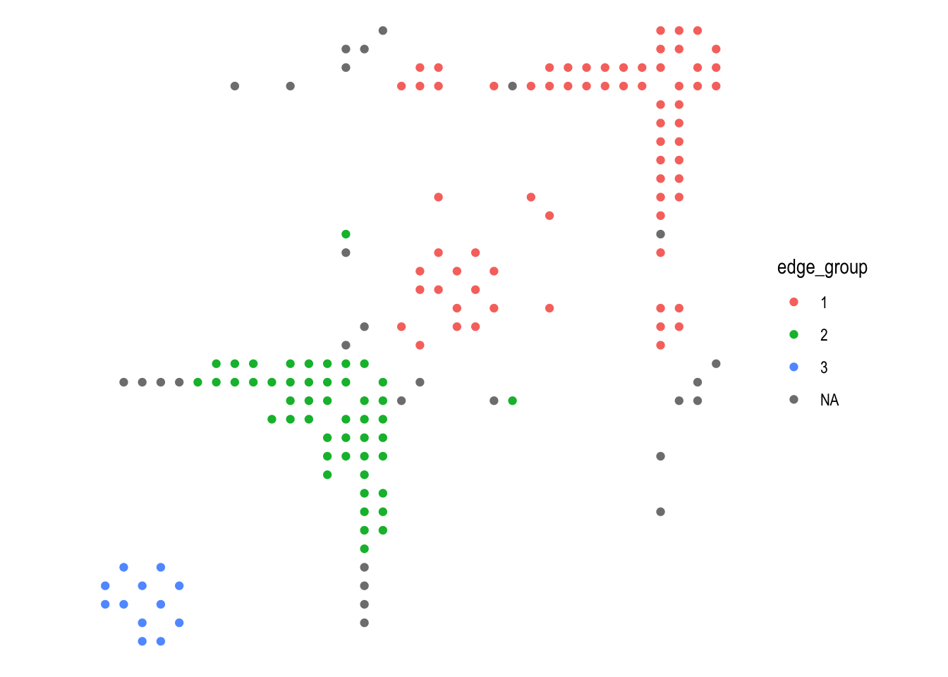
As can be seen in the example above it is often useful to mirror edges to both sides of the diagonal to make the patterns stronger. Highly connected nodes are easily recognizable, without suffering from over-plotting, and by choosing an appropriate ranking algorithm communities are easily visible. In addition to gemo_edge_point() ggraph also provides geom_edge_tile() for a different look.

The fabric layout (originally called biofabric, but I have decided to drop the prefix to indicate it can be used generally), is another layout approach that tries to deal with the problems of over-plotting. It does so by drawing all edges as evenly spaced vertical lines, and all nodes as evenly spaced horizontal lines. As with the matrix layout it is highly dependent on the sorting of nodes, and requires some getting used to. I urge you to give it a chance though, potentially with some help from the website its inventor has set up:

ggraph(graph, 'fabric', sort.by = node_rank_fabric()) + 
  geom_node_range(aes(colour = group), alpha = 0.3) + 
  geom_edge_span(aes(colour = edge_group), end_shape = 'circle') + 
  coord_fixed() + 
  theme(legend.position = 'top')

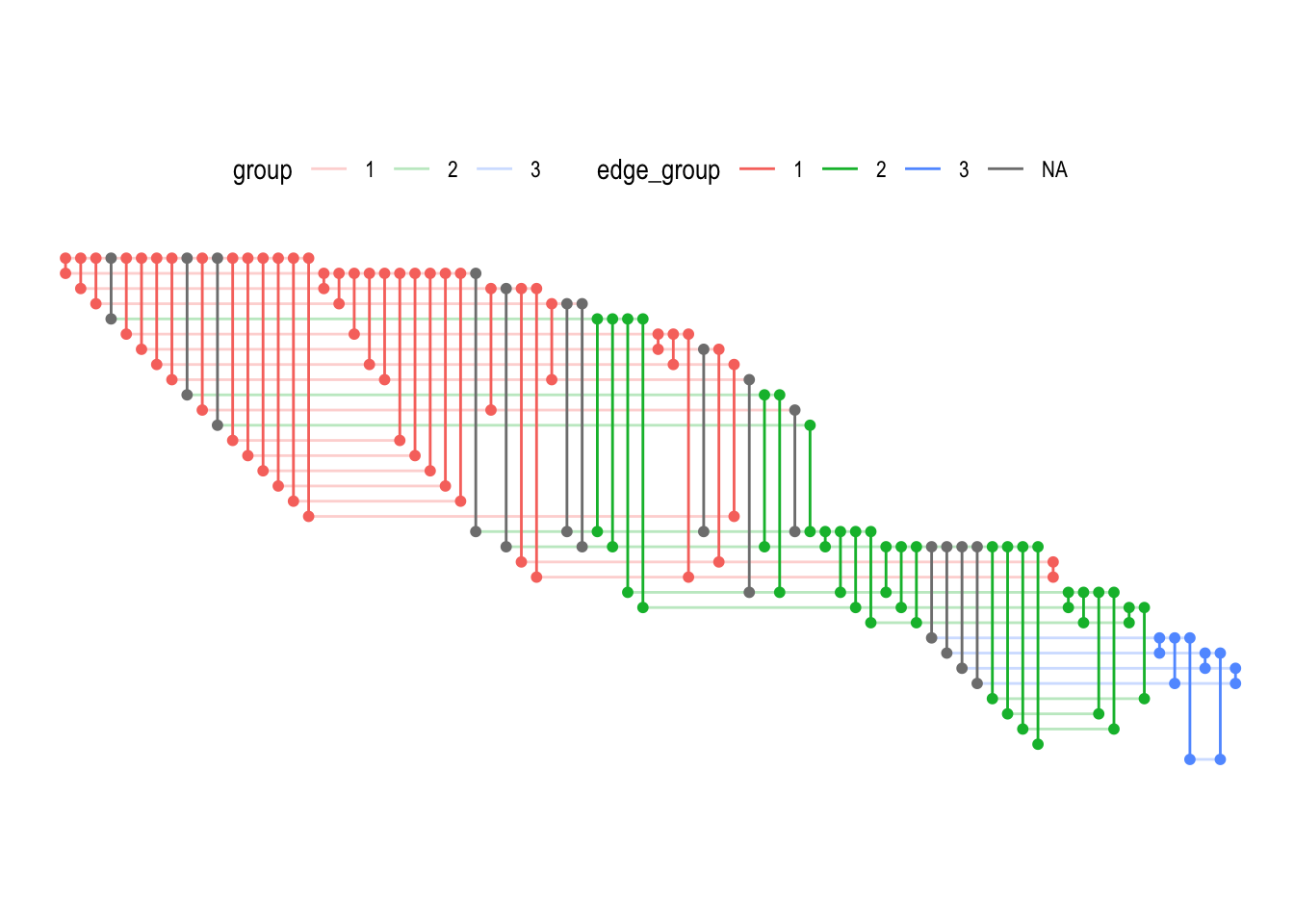
The node_rank_fabric() is the ranking proposed in the original paper, but other ranking algorithms are of course also possible.

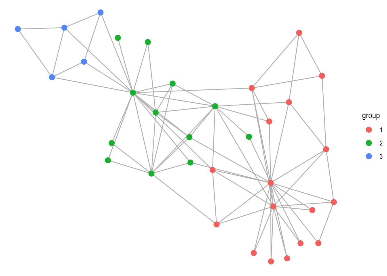
The last new feature in the layout department is that it is now easier to plug in new layouts. First, by providing a matrix or data.frame to the layout argument in ggraph() you can quickly provide a fixed position of the nodes. The same can be obtained by providing an x and y argument to the ‘auto’ layout. Second, you can provide a function directly to the layout argument. The function must take a tbl_graph as input and return a data.frame or an object coercible to one. This means that e.g. layouts defined as physics simulations with the particles package can be used directly:

library(particles)
# Set up simulation
sim <- . %>% simulate() %>% 
  wield(manybody_force) %>% 
  wield(link_force) %>% 
  evolve()

ggraph(graph, sim) + 
  geom_edge_link(colour = 'grey') + 
  geom_node_point(aes(colour = group), size = 3)

Geoms for the people

While ggraph has always included quite a large range of different geoms for showing nodes and edges, this release has managed to add some more. Most importantly, geom_edge_fan() has gained a brother in crime for showing multi-edges. geom_edge_parallel() will draw edges as straight lines but, in the case of multi-edges, will offset them slightly orthogonal to its direction so that there is no overlap. This is a geom best suited for smaller graphs (IMO), but here it can add a very classic look to the plot:

small_graph <- create_notable('bull') %>%
  convert(to_directed) %>%
  bind_edges(data.frame(from = c(1, 2, 5, 3), to = c(2, 1, 3, 2)))

ggraph(small_graph, 'stress') + 
  geom_edge_parallel(end_cap = circle(.5), start_cap = circle(.5),
                     arrow = arrow(length = unit(1, 'mm'), type = 'closed')) + 
  geom_node_point(size = 4)

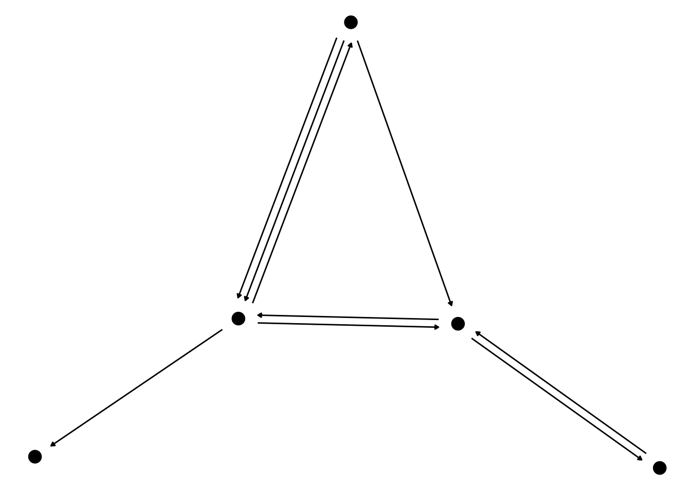
For this edge geom in particular it is often a good idea to use capping to let them end before they reaches the terminal nodes.

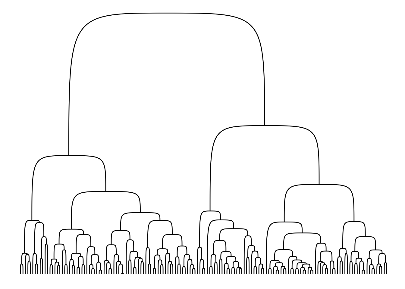
Another edge geom that has become available is geom_edge_bend() which is sort of an organic elbow geom:

ggraph(iris_clust, 'dendrogram', height = height) + 
  geom_edge_bend()

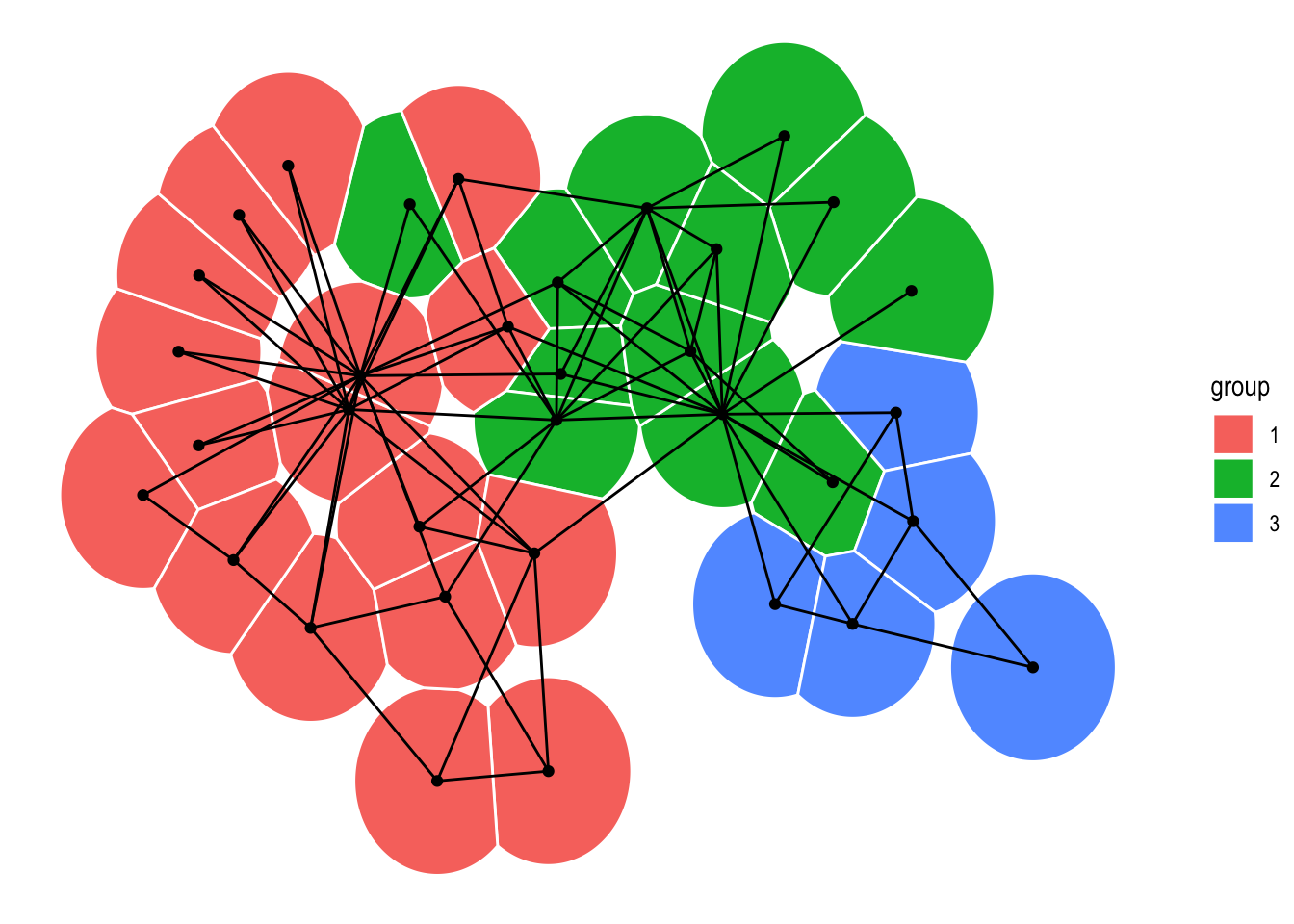
Lastly, in addition to the node and edge geoms shown in the Layout section, geom_node_voronoi() has been added. It is a ggraph specific version of ggforce::geom_voronoi_tile() that allows you to create a Voronoi tessellation of the nodes and use the resulting tiles to show the nodes. As with the ggforce version it is possible to constrain the tiles to a specific radius around the edge making it a great way of showing which nodes dominates certain areas without any problems with over-plotting.

ggraph(graph, 'stress') + 
  geom_node_voronoi(aes(fill = group), max.radius = 0.5, colour = 'white') + 
  geom_edge_link() + 
  geom_node_point()

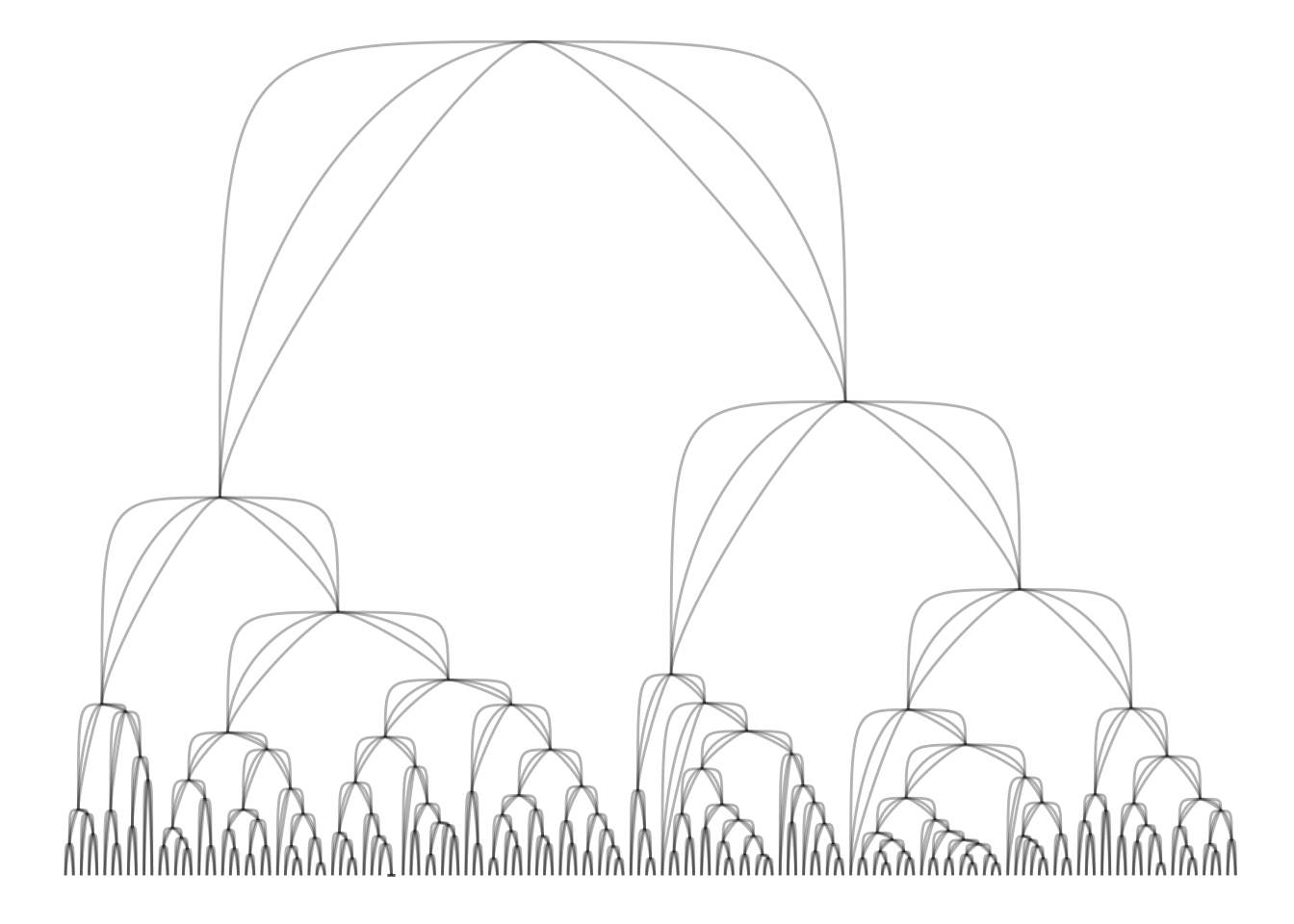
A last little thing pertaining to edge geoms is that many have gained a strength argument, which controls their level of non-linearity (this is obviously only available for non-linear edges). Setting strength = 0 will result in a linear edge, while setting strength = 1 will give the standard look. Everything in between is fair game, while everything outside that range will look exceptionally weird, probably.

ggraph(iris_clust, 'dendrogram', height = height) + 
  geom_edge_bend(alpha = 0.3) + 
  geom_edge_bend(strength = 0.5, alpha = 0.3) + 
  geom_edge_bend(strength = 0.2, alpha = 0.3)

ggraph(iris_clust, 'dendrogram', height = height) + 
  geom_edge_elbow(alpha = 0.3) + 
  geom_edge_elbow(strength = 0.5, alpha = 0.3) + 
  geom_edge_elbow(strength = 0.2, alpha = 0.3)

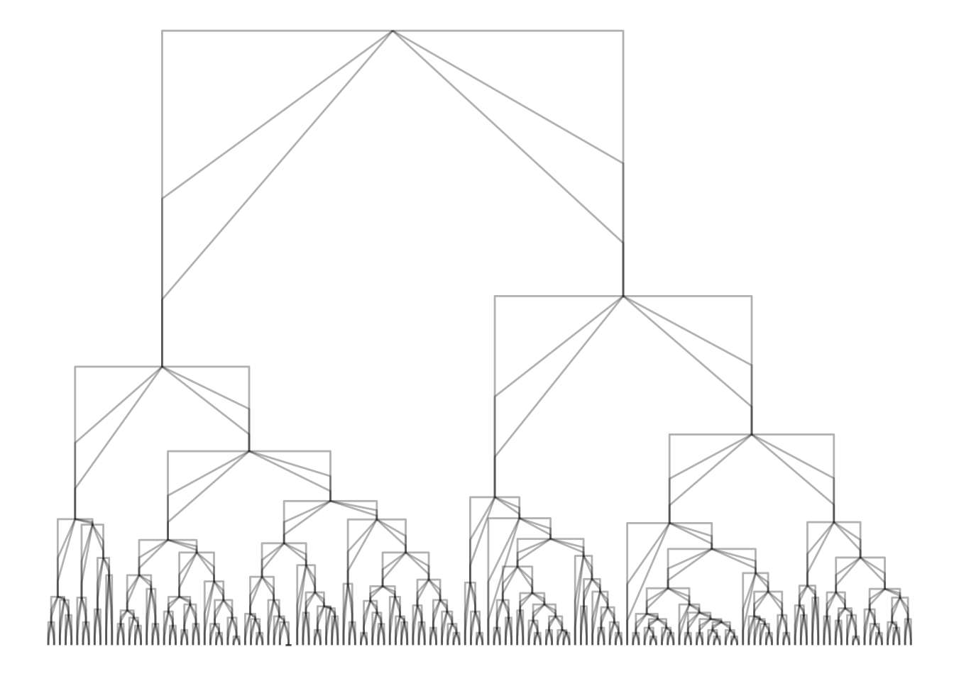
A few geoms have had arguments such as curvature or spread that have had similar purpose, but those arguments have been deprecated in favor of the same argument across all (applicable) geoms.

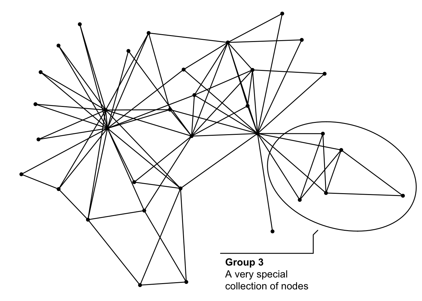
And then one more last thing, but it is really not something new in ggraph. As you can use standard geoms for drawing nodes some of the new features in ggforce is of particular interest to ggraph users. The geom_mark_*() family in particular is great for annotating single, or groups of nodes, and going forward it will be the advised approach:

library(ggforce)
ggraph(graph, 'stress') + 
  geom_edge_link() + 
  geom_node_point() + 
  geom_mark_ellipse(aes(x, y, label = 'Group 3', 
                        description = 'A very special collection of nodes',
                        filter = group == 3))

All the rest

These are the exiting new stuff, but the release also includes numerous bug fixes and small tweaks… Far to many to be interesting to list, so you must take my work for it 😄.

As with ggforce I hope that ggraph never goes this long without a release again. Feel free to flood me with feature request after you have played with the new version and I’ll do my best to take them on.

I’ll spend some time on ggplot2 and grid for now, but still plan on taking a development sprint with patchwork with the intend of getting it on CRAN before the end of this year.