transformr: Age of Spatial
Once again, I gives me great pleasure to announce a new package has joined CRAN. transformr is the spatial brother of tweenr and as with the tweenr update a few months ago, this package is very much driven by the infrastructural needs of gganimate. It is probably the last piece needed before I can begin preparing gganimate for CRAN, so if you are waiting for that there is indeed reason for celebration.
Becoming Spatial
As written above, transformr is tweenr for spatial data (spatial being used in a very broad sense as any data that is partly coordinates). To understand what this means we’ll briefly have to touch on a core concept of tweenr. What is never said out loud, but generally implied, is that tweenr treats all columns of the data frame as independent. This is generally a sound principle as you don’t want values from other columns to influence how e.g. the colour transitions between black and blue. As far as spatial is concerned, this approach also works fine as each row in the data frame encodes a single independent point in space or if there’s a one-to-one mapping between points in a polygon. Alas, the devil’s in the detail, and tweenr breaks down in magnificent ways if you try to tween between more complicated and heterogeneous shapes, e.g. a star and a circle. This is not something unique to tweenr, mind you, d3.js also has this limitation. The problems in d3 led Noah Veltman to develop the flubber javascript library. His reasons for developing it is succintly described in the animation below, grabbed from the readme of flubber

The Trials of the Polygon
So, what’s the deal with polygons exactly. Why don’t they just do as you expect them to and morph naturally from one to the other. That sad state of affair is that there are multiple reasons for that:
- There might be discrepancy between the number of points that make up the two polygons. This may lead to part of the shape simply appearing or disappearing at the start or end of the tween.
- The winding of the polygons may have a different angular offset and/or direction. This means that the tween will include rotatation and/or inversion, something that is often undesirable.
- There may be a discrepancy in the number of polygons that make up the two shapes you tween between and/or a discrepancy between the number of holes. As with 1. this may lead to parts of the shapes suddenly appearing or disappearing during the tween.
Running the Gauntlet
transformr tries to solve the three problems above in much the same way as flubber does, at least conceptually. There are enough differences between how Javascript and R (as well as d3 and tweenr) works with data, that I decided to only take the ideas behind flubber and implement them in my own way, in a manner fitting for R, rather than doing a direct port of the library. This means that you cannot expect the two libraries to behave equivalently. Below is, at a very high level, what transformr does to address the 3 problems outlined above:
- Points are added along the edges of the shape with the fewest corners until the number of points matches between the shapes. Points are added so that long edges will be divided more often than short edges in order to even out the edge lengths of the final shape. Further, if any shape has fewer than a given number of corners, points will be added (following the same strategy) until the number of corners is reached.
- After the number of points are evened out, the winding direction is matched between the shapes (as clockwise), and the last shape is rotated until the squared distance between point pairs of the two shapes is minimised.
- This is adressed first (but is the least prevalent problem so it is mentioned last). If there are different number of polygons in the two states you wish to tween between, the polygons in the state with the fewest polygons is cut until the number matches. Once again, the cuts are distributed so that large polygons are cut more often than small. After the cutting, polygons between the states are matched by minimising distance and area difference. If there are differences in the number of holes in the matched polygons zero-area holes are inserted at the gravitational center of the polygon with the fewest holes until the number matches.
The Ways of the Transformr
At this point we have only talked about shapes (and polygons), so let’s get a bit more concrete. transformr currently recognises three data types: polygons, paths, and simple features. Polygons encompass simple polygons as well as polygons with any number of holes. Paths can be either single or multipaths. Simple features as implemented by the sf package are supported, currently covering the (multi)point, (multi)path, and (multi)polygon types.
In terms of tween type support, transformr currently extends the tween_state() API from tweenr but support for the other types of tweeners will be added with time.
Some Examples
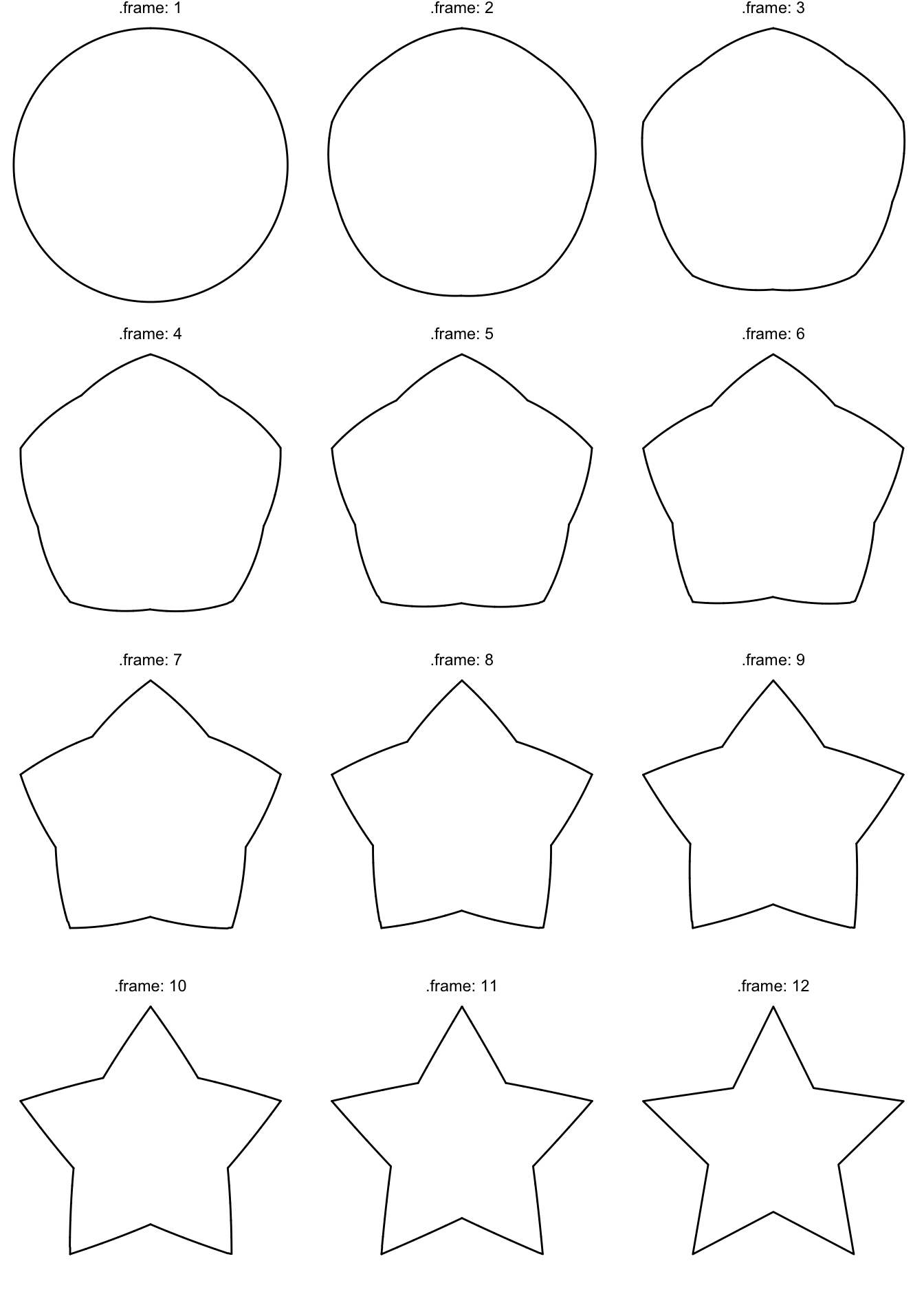
At this point an example is probably in order. We’ll start with what we first identified as a problematic case: morphing between a circle and a star:
library(transformr)
library(ggplot2)

# Helpers included in transformer
circle <- poly_circle()
star <- poly_star()

# The data is a simple data.frame as you would feed into ggplot2
head(star)
## x y id
## 1 0.000000e+00 1.0000000 1
## 2 2.938926e-01 0.4045085 1
## 3 9.510565e-01 0.3090170 1
## 4 4.755283e-01 -0.1545085 1
## 5 5.877853e-01 -0.8090170 1
## 6 6.123234e-17 -0.5000000 1# We use tween_polygon to morph between the two
morph <- tween_polygon(circle, star,
ease = 'linear',
id = id,
nframes = 12)
# You get back a data.frame with the same special columns as with tweenr
head(morph)## x y id .id .phase .frame
## 1 0.00000000 1.0000000 1 1 raw 1
## 2 0.01745241 0.9998477 1 1 raw 1
## 3 0.03489950 0.9993908 1 1 raw 1
## 4 0.05233596 0.9986295 1 1 raw 1
## 5 0.06975647 0.9975641 1 1 raw 1
## 6 0.08715574 0.9961947 1 1 raw 1# Let's see the result
ggplot(morph) +
geom_polygon(aes(x = x, y = y, group = id), fill = NA, colour = 'black') +
facet_wrap(~.frame, labeller = label_both, ncol = 3) +
theme_void()
What would happen if we upped the stakes a bit? Let’s try with a star with a hole, morphing into three circles:
circles <- poly_circles()
star_hole <- poly_star_hole()

morph <- tween_polygon(circles, star_hole,
                       ease = 'linear',
                       id = id,
                       nframes = 12,
                       match = FALSE)

ggplot(morph) +
  geom_polygon(aes(x = x, y = y, group = id), fill = NA, colour = 'black') +
  facet_wrap(~.frame, labeller = label_both, ncol = 3) +
  theme_void()
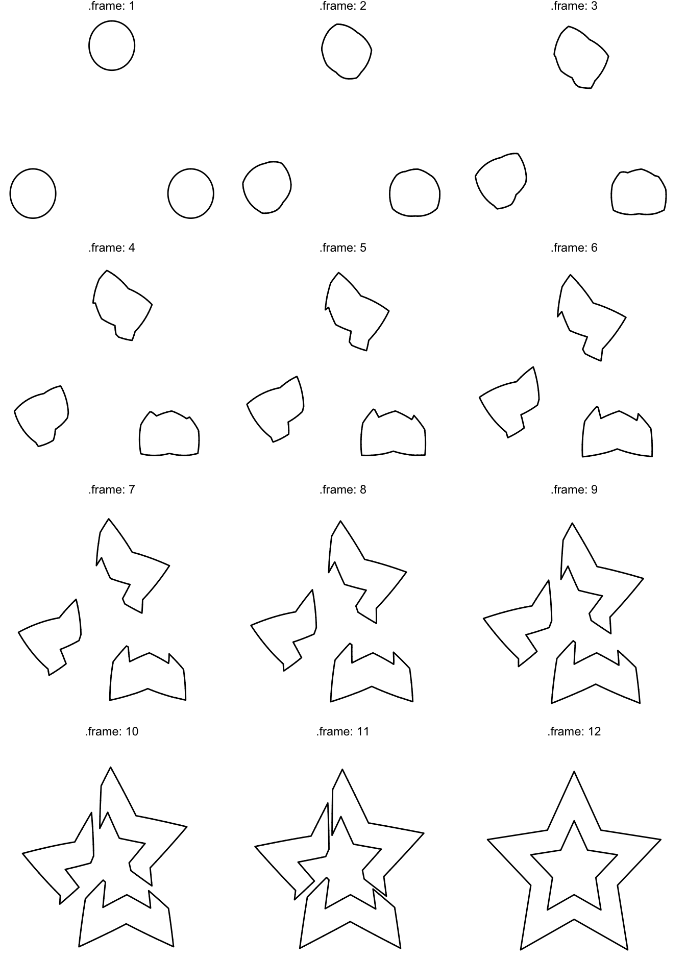
We introduced a new argument in tween_polygon() here. match is used to define whether polygons are matched by the value of id or whether all polygons in the first state should somehow morph into all polygons in the last state. If we set match = TRUE, we can use the enter and exit argument to define what should happen to unmatched polygons
morph <- tween_polygon(circles, star_hole,
                       ease = 'linear',
                       id = id,
                       nframes = 12,
                       match = TRUE,
                       exit = function(.x) transform(.x, x = mean(x), y = mean(y)))

ggplot(morph) +
  geom_polygon(aes(x = x, y = y, group = id), fill = NA, colour = 'black') +
  facet_wrap(~.frame, labeller = label_both, ncol = 3) +
  theme_void()
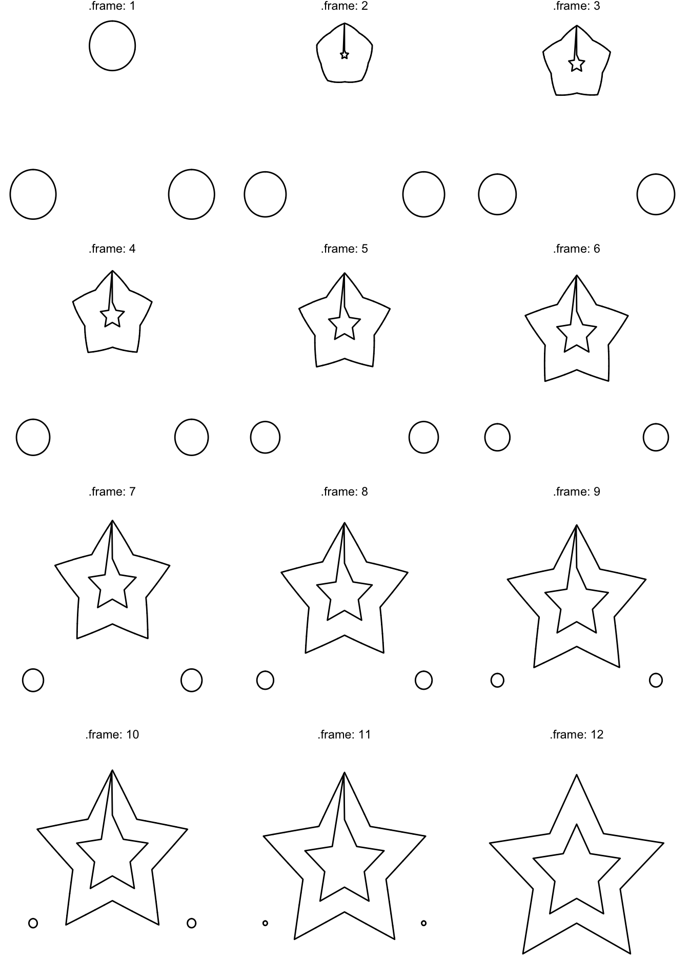
You’ll see a weird glitch above with the hole in the star reaching out to the edge, but this is simply ggplot2 not knowing how to deal with holed polygons in geom_polygon() — I’ll handle that in another post…
What is not shown above is that transformr and tween_polygon() works well together with keep_state() from tweenr and that it is pipe-able, but if you are used to tween_state() this will all come natural…
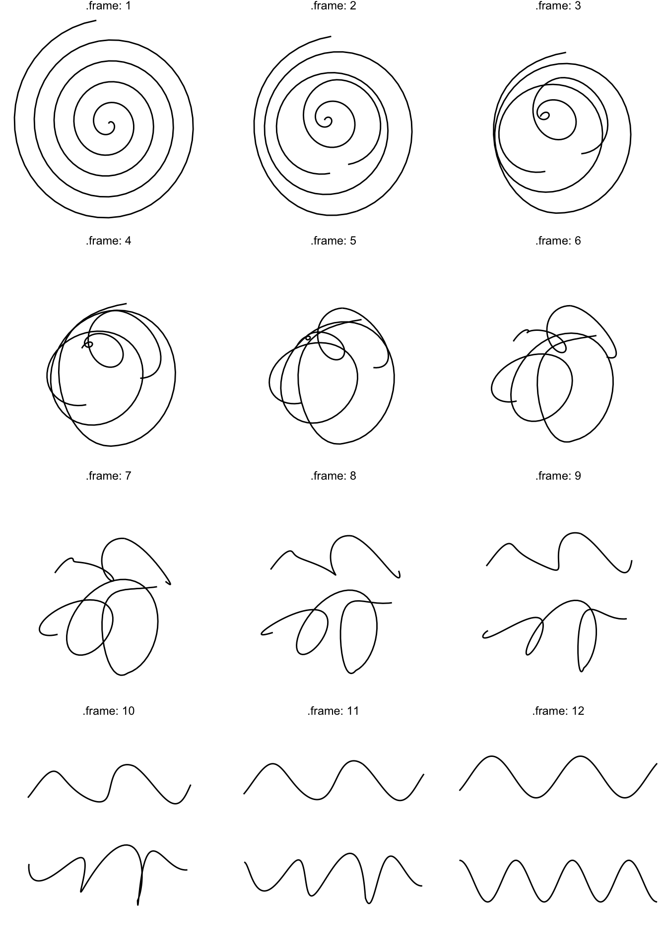
While path and sf morphing works in much the same way as shown above, I’ll quickly show case it for completeness:
spiral <- path_spiral()
waves <- path_waves()

morph <- tween_path(spiral, waves,
                    ease = 'linear',
                    nframes = 12,
                    id = id,
                    match = FALSE)

ggplot(morph) +
  geom_path(aes(x = x, y = y, group = id), colour = 'black') +
  facet_wrap(~.frame, labeller = label_both, ncol = 3) +
  theme_void()
circle_st <- sf::st_sf(geometry = sf::st_sfc(poly_circle(st = TRUE)))
north_carolina <- sf::st_read(system.file("shape/nc.shp", package = "sf"),
                              quiet = TRUE)
north_carolina <- st_normalize(sf::st_combine(north_carolina))
north_carolina <- sf::st_sf(geometry = sf::st_sfc(north_carolina))

morph <- tween_sf(north_carolina, circle_st,
                  ease = 'linear',
                  nframes = 12)

ggplot(morph) +
  geom_sf(aes(geometry = geometry), colour = 'white', fill = 'black', size = .1) +
  facet_wrap(~.frame, labeller = label_both, ncol = 3) +
  coord_sf(datum = NULL) +
  theme_void()
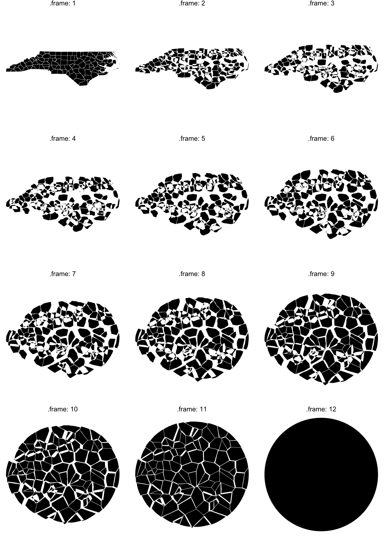
As can be seen, transformr can handle most of the things you choose to to throw at it, when it comes to morphing between different shapes. It is used under the hood in gganimate to power polygon, path, and sf geom transitions (and derivatives thereof), but can just as well be used directly in the same way as tweenr can…
I do hope you’ll enjoy transformr either simply through the magic of gganimate or by playing with it directly — the results can be quite mesmerizing…