Let it flow, let it flow, let it flow

simulation

particles

announcement

network

February 22, 2018

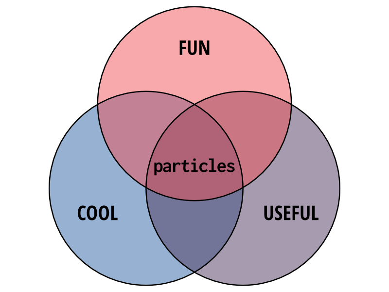
I got a new package on CRAN! It’s called particles and it sits right in the perfect intersection of fun, cool, and useful. If you don’t believe me, have a look at the Venn diagram below — charts don’t lie!

So what is this all about?

particles is an R implementation of The d3-force algorithm developed by Mike Bostock and can be used to simulate many different types of interactions between particles and the world. While particles can be used as a simple physics engine it has not been developed with this in mind and accuracy, in terms of how well it behaves like the physical world, has not been a main priority during development.

In it’s essence particles provides a way of defining a set of spherical or dimensionless object, potentially connected with each other, a world governed by a set of rules, and then set the objects free in the world and see how they behaves. The use cases for this are many, and include network visualisation, generative art, animation, and - most importantly - fun!

particles is build on top of tidygraph and uses it as the main representation of the particles and their relations. Even so, there is no need to be experienced in network analysis and manipulation. particles can easily be used without any of the objects being connected with each other and the objects can thus be thought of as stored in a simple data frame.

Setting up a simulation

Central to the use of particles is the simulation, that is, setting the objects free in the world you’ve defined. There are several parts to a simulation:

A description of the objects you wish to simulate
An initialisation of the position and velocity of the objects
A specification of how the simulation progress over time (e.g. a cooling, letting the simulation slowly stabilise)
A number of forces and constraints that governs how the objects behave in the system
A specification of how many iterations the simulation should evolve

All of these steps can be specified using dedicated verbs and piped together. Let’s look at an example:

library(particles)
library(tidygraph)

sim <- create_ring(10) %>% 
  simulate(velocity_decay = 0.6, setup = petridish_genesis(vel_max = 0)) %>% 
  wield(link_force) %>% 
  wield(manybody_force) %>% 
  impose(polygon_constraint, 
         polygon = cbind(c(-100, -100, 100, 100), c(-100, 100, 100, -100))) %>% 
  evolve(100)

So what’s going on here? First we create a tbl_graph using the create_ring() function from tidygraph, which basically creates a circular graph. Then we use it to create a simulation using the simulate() function. In there we can set how fast the velocity decays over time, as well how particles should be initialised. We use the petridish_genesis() to place the particles randomly on a disc. Then we begin to define the forces that makes up the simulation using the wield() function. We first add a link force that makes connected particles attract each other, and then a manybody force that pushes particles away from each others (unless the strength is set to a positive value in which case it works like gravity, attracting particles to each other). We also adds a constraint to the system using the impose() function. Here we defines that particles must remain inside a 200x200 square.

The distinction between forces and constraints are a bit vague but generally forces will adjust the velocity of particles while constraints defines hard boundaries for the position and velocity of the particles.

Lastly we set the simulation to run for 100 iterations. If we did not specify a number of iterations the simulation would run until it had cooled down (which happens after 300 iterations using the default settings). We now have a simulation that has progressed a bit:

sim
#> A particle simulation:
#> * 10 particles
#> * 2 Forces
#>   - link_force
#>   - manybody_force
#> * 1 Constraints
#>   - polygon_constraint
#> * 100 Evolutions

We could say that that was it and maybe plot it:

library(ggraph)
ggraph(as_tbl_graph(sim)) + 
  geom_edge_link() + 
  geom_node_point() + 
  theme_graph()

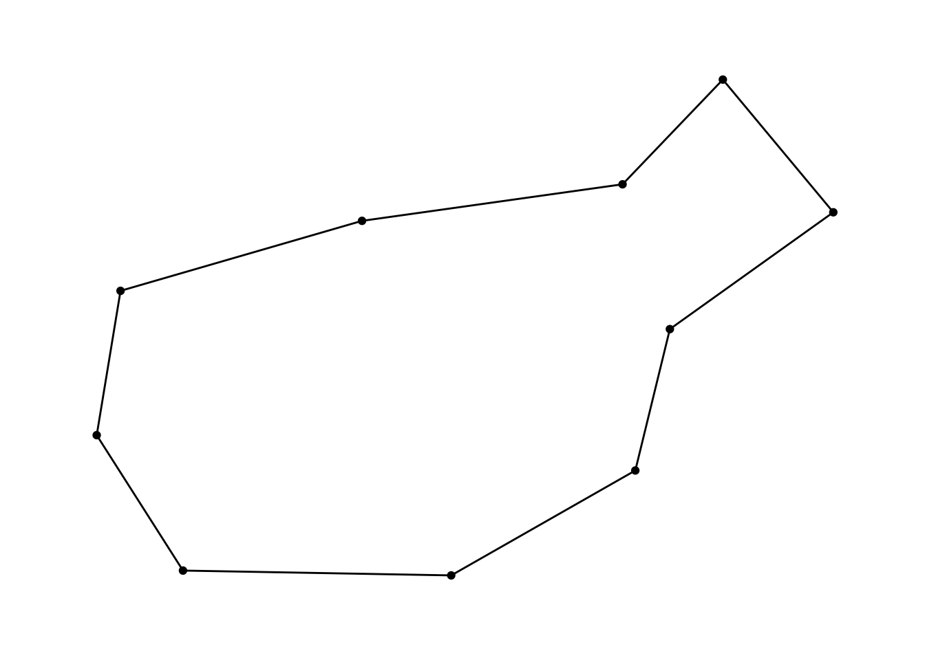
(as we can see the simulation has almost unwinded the ring from its initial random state)

We could also change the simulation somehow and iterate some more on it:

sim <- sim %>% 
  unwield(2) %>% 
  wield(manybody_force, strength = 30) %>% 
  reheat(1) %>% 
  evolve()

ggraph(as_tbl_graph(sim)) + 
  geom_edge_link() + 
  geom_node_point() + 
  theme_graph()

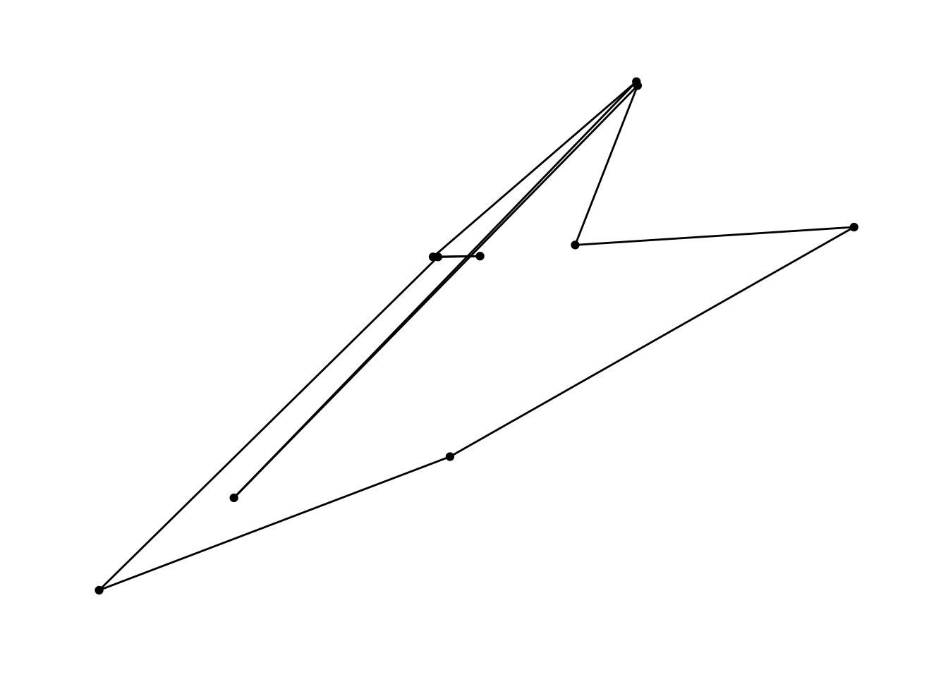
Let’s unpack this. First we remove the second force (the repulsive manybody force) and then we add a new manybody force that attracts instead (these two steps could also have been done in one using rewield()). Then we heat up the system again (setting alpha back to the original value) and let it evolve until it has cooled down. The result is a struggle between the link force and the manybody force over dominance of the system.

Tidy eval

Many of the different forces and constraints let you set parameters on a per particle or per connection basis - e.g. for the link force discussed above we could let the strength of the force be related to the weight of the edge. particles let you reference node and edge variables directly when specifying the force or constraint, e.g.

sim <- play_islands(3, 10, 0.6, 3) %>% 
  mutate(group = group_infomap()) %>% 
  activate(edges) %>% 
  mutate(weight = ifelse(.N()$group[to] == .N()$group[from], 1, 0.25)) %>% 
  simulate() %>% 
  wield(link_force, strength = weight, distance = 10/weight) %>% 
  evolve()

ggraph(as_tbl_graph(sim)) + 
  geom_edge_link(aes(width = weight), alpha = 0.3, lineend = 'round') + 
  geom_node_point() + 
  theme_graph() + 
  theme(legend.position = 'none')

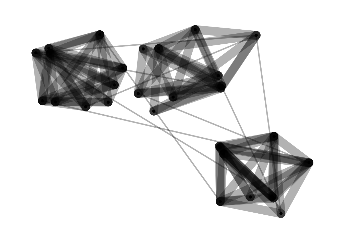
The nice thing about using node and edge variables is that particles keeps track of them and if you change them the force will get retrained:

sim <- sim %>% 
  activate(edges) %>% 
  mutate(weight = 1) %>% 
  reheat(1) %>% 
  evolve()

ggraph(as_tbl_graph(sim)) + 
  geom_edge_link(aes(width = weight), alpha = 0.3, lineend = 'round') + 
  geom_node_point() + 
  theme_graph() +
  theme(legend.position = 'none')

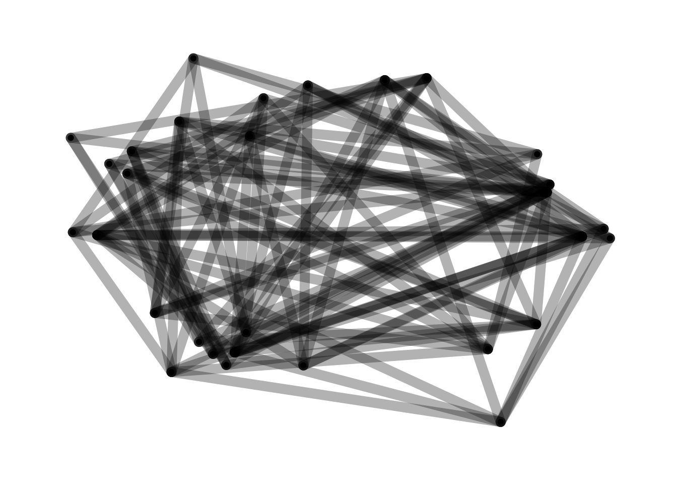
Consult the documentation of each force and constraint to see which parameters that are tidy evaled.

Note that we are able to manipulate the underlying tbl_graph directly using active(), mutate(), and filter() - particles defines a subset of the verbs defined in tidygraph/dplyr

Iteration callback

Sometimes you are more interested in the process than the end point. In that case you might want to look at the state of the simulation at each step it goes through. Luckily, the evolve() function comes with a powerful callback mechanism that allows you to do all sorts of things. If the callback function returns a simulation object it will replace the current simulation, otherwise the return value will be discarded and the side-effects, such as plots, will be the only effect of it. As you can imagine you can do many things with this capability, such as removing or adding new particles and connections, or changing forces midway. If the callback plots the current state it can be used directly with the animation package to produce animated views of your simulation. Lastly, it can be used to record the state so the it can easily be retrieved later on. For this you can use the predefined record() function:

volcano_field <- (volcano - min(volcano)) / diff(range(volcano)) * 2 * pi
sim <- create_empty(1000) %>% 
  simulate(alpha_decay = 0, setup = aquarium_genesis(vel_max = 0)) %>% 
  wield(reset_force, xvel = 0, yvel = 0) %>% 
  wield(field_force, angle = volcano_field, vel = 0.1, xlim = c(-5, 5), ylim = c(-5, 5)) %>% 
  evolve(100, record)

traces <- data.frame(do.call(rbind, lapply(sim$history, position)))
names(traces) <- c('x', 'y')
traces$age <- rep(100:1, each = 1000)
traces$particle <- rep(1:1000, 100)

ggplot(traces) +
  geom_path(aes(x, y, group = particle, alpha = age), size = 0.1) + 
  theme_void() + 
  theme(legend.position = 'none')

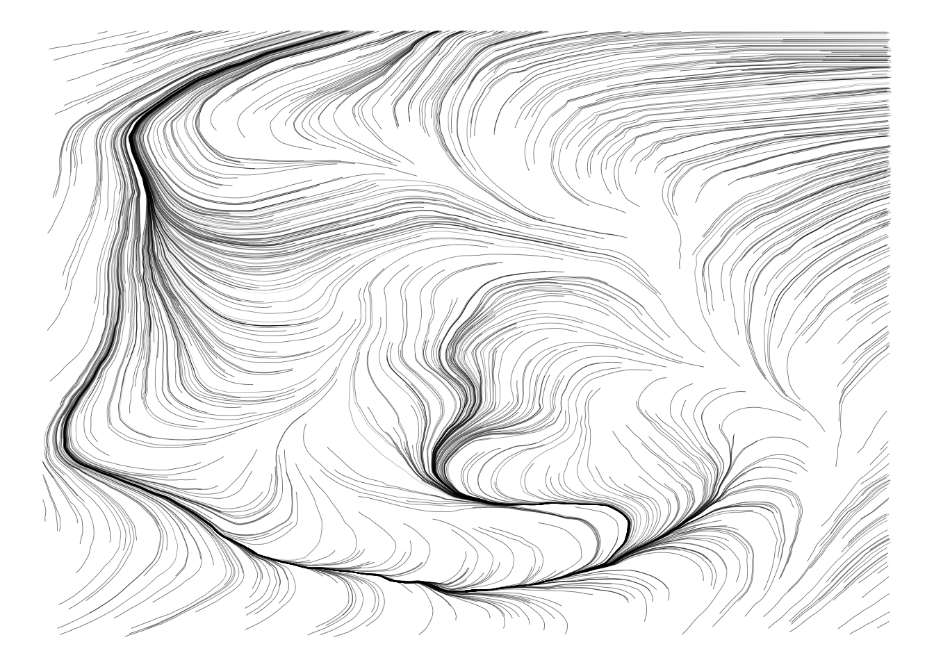
In this example we define a field force based on our beloved volcano data set. The field force applies a velocity based on a given vector field. We define that the simulation has no cooling (alpha_decay = 0) and that the particles should be placed randomly in a rectangle. Besides the field force we also add a reset force that sets the velocity to zero in each iteration so that the vector field does not accumulate. When all this is done we run the simulation for 100 iterations and saves each state with the record() function.

To get the plot we extract the positions from each iteration and simply plots the trajectory of each particle.

But lines are all fine and great — let’s see an animation instead:

create_empty(1000) %>% 
  simulate(alpha_decay = 0, setup = aquarium_genesis(vel_max = 0)) %>% 
  wield(reset_force, xvel = 0, yvel = 0) %>% 
  wield(field_force, angle = volcano_field, vel = 0.1, xlim = c(-5, 5), ylim = c(-5, 5)) %>% 
  evolve(100, function(sim) {
    p <- ggplot(as_tibble(sim)) + 
      geom_point(aes(x, y), size = 0.25) + 
      theme_void()
    plot(p)
  })

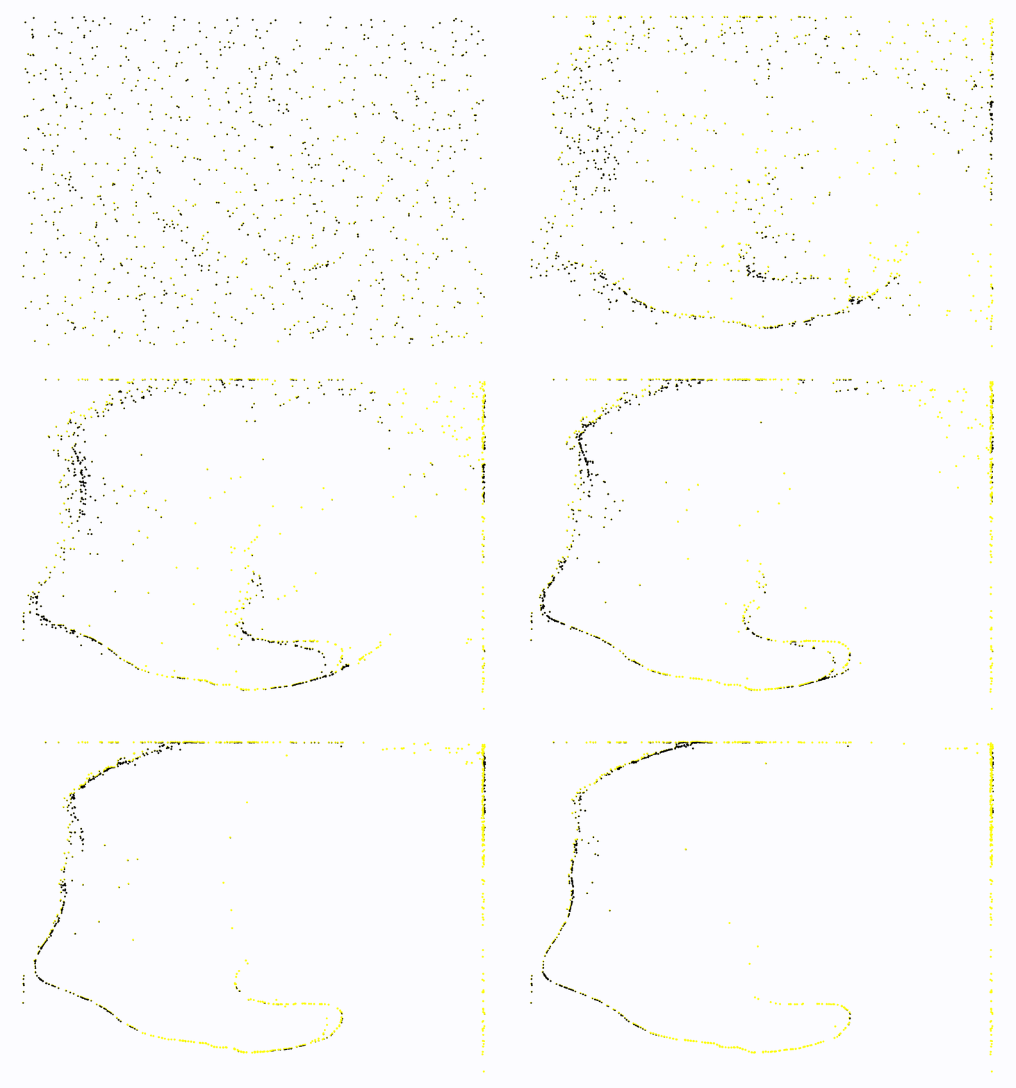
#> A particle simulation:
#> * 1000 particles
#> * 2 Forces
#>   - reset_force
#>   - field_force
#> * 0 Constraints
#> * 100 Evolutions

Summing up

Hopefully you have gotten a taste of what is possible with particles, but there are many more options and possibilities. The package is developed both for practical use and for having fun — with luck you can do both simultaneously.