I am very pleased to tell you that the next version of tidygraph (1.1) is now available on CRAN. This is not a bug-fix release, nor a change-it-all release, but rather a more-of-it-all release, and in this post I’m going to tell you all about it.
The idea of tidygraph
Before we enter the goldmine of new features that makes this release I’m going to talk a bit about my reasons for making tidygraph and what I want it to become. These ideas have been rummaging in my head for a while and has taken more form as I prepared for my RStudio::conf 2018 talk. They will probably be fleshed out even more in a (series of) blog post(s), or — dare I say — a book, but you’ll get the earliest version of it here…
Network analysis is daunting… Sure, have you spend the better part of your life working with it (I haven’t) it might seem common nature, but for most people it will be an area they enter late, unprepared, and already well-versed in the manners of rectangular data analysis. For many, the instinct will be to quickly produce a plot, which will often end up creating very little insight due to the curse of the hairball, and they will leave the world of network analysis with a sense of broken promises. While all of this sounds overtly melodramatic, I honestly feel that the tools we use to do network analysis can do better in guiding the user towards a meaningful network analysis workflow and I hope that tidygraph (and ggraph) will prove to be a decent attempt at that.
With tidygraph I set out to make it easier to get your data into a graph and perform common transformations on it, but the aim has expanded since its inception. The goal of tidygraph is to empower the user to formulate complex questions regarding relational data as simple steps, thus enabling them to retrieve insights directly from the data itself. The central idea this all boils down to is this: you don’t have to plot a network to understand it. While I absolutely love the field of network visualisation, it is in many ways overused in data science — especially when it comes to extracting knowledge from a network. Just as you don’t need a plot to tell you which car in a dataset is the fastest, you don’t need a plot to tell you which pair of friends are the closest. What you do need, instead of a plot, is a tool that allow you to formulate your question into a logic sequence of operations. For many people in the world of rectangular data, this tool is increasingly dplyr (and friends), and I do hope that tidygraph can take on the same role in the world of relational data.
This is not just about preparing your data for a plot — this is about answering questions.
I really just want to read about the new features
With the pompous manifesto out of the way, I’ll get on with describing what the new release brings to the table. I’ll not spend time describing small tweaks and bug fixes and instead focus on what I think are the important parts of this release.
More algorithms
In order to understand networks we are often required to use complex algorithms to assess e.g. the importance of different nodes on the topology of the network. tidygraph approaches this need by taking the idea of dplyr::n() and turbocharging it. As with n() all tidygraph algorithms knows the context in which they are called, so there is no need to specify the graph, nodes, and/or edges the algorithm should be applied to, and you can always expect an output that is directly usable within a mutate call. In v1.0 almost all of igraphs own algorithms had been wrapped in this way, and this version adds support for a lot of algorithms from other packages. In order to keep the dependencies at a minimum all of these packages are only suggested and it is up to the user to install them to get access to the features:
Node ranking
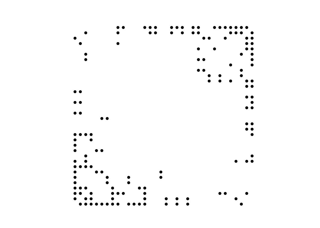
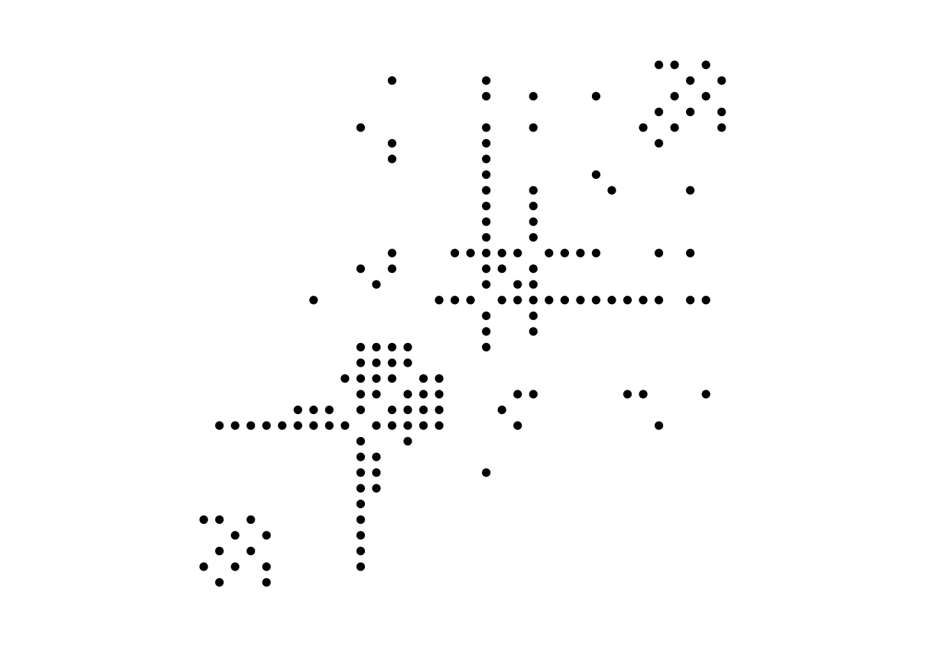
Often, especially when visualising networks with certain layouts, the order in which the nodes appear will have a huge influence on the insight you can get out (e.g. matrix plots and arc diagrams). The node_rank_*() family of algorithms have been introduced to provide different ways of sorting nodes so that closely related nodes are positionally close. As there is often not a single correct answer to this endeavor, there’s a lot of different algorithms that may provide different insights into your network. Many of them are based on the seriation package, and the vignette provided therein serves as a nice introduction to the different algorithms:
library(tidygraph)
library(ggraph)

graph <- create_notable('zachary') %>%
  mutate(ranking = node_rank_leafsort())

ggraph(graph, 'matrix') +
  geom_edge_point(mirror = TRUE) +
  theme_graph() +
  coord_fixed()

ggraph(graph, 'matrix', sort.by = ranking) +
  geom_edge_point(mirror = TRUE) +
  theme_graph() +
  coord_fixed()

As you can see, interpretable patterns can appear once the nodes are arranged in the right fashion.
Centrality
Centrality scores were not badly supported in the last version as all of igraphs different algorithms were implemented. This version adds 19(!) new ways to define the notion of centrality along with a manual version where you can mix and match different distance measures and summation strategies opening up the world to even more centrality scores. All of this wealth of centrality comes from the netrankr package that provides a framework for defining and calculating centrality scores. If you use centrality measures somewhere in your analysis I cannot recommend the vignettes provided by netrankr enough as they provide a fundamental intuition about the nature of such measures and how they can/should be used.
Node measures
While centrality is often used as a measure of node importance it is often done so wrongly. While centrality measures are often good at picking out the top central nodes, the numbers themselves have little interpretability. Furthermore they are often bad at distinguishing the middle bulk of nodes from each other. In order to provide a more numerical measure of node importance the new version of tidygraph provides an interface to the algorithms provided by the NetSwan and influenceR packages. NetSwan provides different ways to measure node importance as the impact on the network when the node is removed, while the influenceR provides a more diverse set of algorithms measuring e.g. access to structural holes and effect on cohesiveness.
The coming of morphers
The morph(), unmorph(), and crystallise() verbs were probably one of the ideas I was most proud of with the release of tidygraph. I don’t know how much they have taken on, but to me they are an essential part in formulating network questions as tidy piping operations. If you haven’t used them, then essentially they allow you to perform a temporary topology change on your graph, perform some actions on it, and then switch back to the old topology, keeping all the information added to the nodes and edges.
With the new version the number of morphers have grown (morphers are the functions defining the topological change and has a to_*() naming scheme) and a new related verb has appeared. The new morphers are to_directed, to_undirected, to_unfolded_tree, and to_hierarchical_clusters. The first two are self-explanatory, the third is akin to igraph::unfold_tree , while the fourth is for deriving hierarchies from hierarchical community detection algorithms (currently walktrap, leading_eigen, and edge_betweenness).
The new verb is convert which will simply convert the graph directly to the new topology, loosing any ties it had with the old graph. Thus, you can not unmorph() a converted graph. If the morpher returns a list of graphs only one will be chosen (defaults to the first) — if you need them all you’ll still need to use morph(), followed by crystallise(). The new verb is a nice way to allow any morpher to be used for both temporary and lasting conversions, thus reducing both my development work and the cognitive load on using tidygraph.
Grab bag
A lot of smaller refinements have been added as well that deserves a quick mention:
-
Two new pipes have been added that performs the
activatestep implicitly.%N>%will activate nodes and%E>%will activate edges. I generally recommend using the explicit approach, but for quick one-liners (e.g. when iteration on aggraphplot), these two new pipes can be handy. -
Added a
with_graphfunction that allows you to call the different algorithms outside of the verbs, e.g.with_graph(gr, group_infomap()). Remember thattbl_graphobjects are fully qualifiedigraphobjects as well, so many of the algorithms could be called using the igraph function as well (igraph::cluster_infomap(gr)) -
Speaking of grouping algorithms, all of these have been modified so the indexing of groups will be ensured to be in decreasing order of size. You can thus always be sure that the nodes indexed with
1will be members of the largest group. -
Added
edge_is_from|to|between|incidentto help identify edges that runs between specific sets of nodes.
More to come…
This is what I had to say about the present release. Still, I have many plans for the network analysis tooling in R. The next thing you’ll probably see is a new version of ggraph with many internal changes that incorporates tidygraph into the backbone with great effects. I’m also looking into providing bindings to the SNAP C++ library for highly efficient network handling. This binding will be complimentary to tidygraph and I have no plans on moving away from igraph as a backend — both libraries have different things to offer. Lastly, I still have many ideas for improving tidygraph that has yet to come to fruition. The evasive idea of somehow incorporating network modelling still lurks in the back of my head, and I have ideas for a couple of new verbs that I’m still figuring out how should really work.
Take care…